Exercises
Getting started
Welcome to SALMON Exercises!
In these exercises, we explain the use of SALMON from the very beginning, taking a few samples that cover applications of SALMON in several directions. We assume that you are in the computational environment of UNIX/Linux OS. First you need to download and install SALMON in your computational environment. If you have not yet done it, do it following the instruction, download and Install and Run.
As described in Install and Run, you are required to prepare at least an input file and pseudopotential files to run SALMON. In the following, we present input files for several sample calculations and provide a brief explanation of the input keywords that appear in the input files. You may modify the input files to execute for your own calculations. Pseudopotential files of elements that appear in the samples are also attached. We also present explanations of main output files.
We present 10 exercises.
First 3 exercises (Exercise-1 ~ 3) are for an isolated molecule, acetylene C2H2. If you are interested in learning electron dynamics calculations in isolated systems, please look into these exercises. In SALMON, we usually calculate the ground state solution first. This is illustrated in Exercise-1. After finishing the ground state calculation, two exercises of electron dynamics calculations are prepared. Exercise-2 illustrates the calculation of linear optical responses in real time, obtaining polarizability and photoabsorption of the molecule. Exercise-3 illustrates the calculation of electron dynamics in the molecule under a pulsed electric field.
Next 2 exercises (Exercise-4 ~ 5) are for a crystalline solid, silicon. If you are interested in learning electron dynamics calculations in extended periodic systems, please look into these exercises. Since ground state calculations of small unit-cell systems are not computationally expensive and a time evolution calculation is usually much more time-consuming than the ground state calculation, we recommend to run the ground and the time evolution calculations as a single job. The following two exercises are organized in that way. Exercise-4 illustrates the calculation of linear response properties of crystalline silicon to obtain the dielectric function. Exercise-5 illustrates the calculation of electron dynamics in the crystalline silicon induced by a pulsed electric field.
Exercise-6 is for an irradiation and a propagation of a pulsed light in a bulk silicon, coupling Maxwell equations for the electromagnetic fields of the pulsed light and the electron dynamics in the unit cells. This calculation is quite time-consuming and is recommended to execute using massively parallel supercomputers. Exercise-6 illustrates the calculation of a pulsed, linearly polarized light irradiating normally on a surface of a bulk silicon.
Exercise-7 ~ 8 are for the linear response and the pulsed electromagnetic field calculation over the metallic nanosphere solving the time-dependent Maxwell equations, where the materials are expressed by dielectric function. The calculation method is the Finite-Difference Time-Domain (FDTD).
Final exercises (Exercise-9 ~ 10) are for geometry optimization and Ehrenfest molecular dynamics based on the TDDFT method for a single water molecule under periodic boundary condition. Currently, these are trial functions. We omit the explanations,but the input keywords are explained in List of all input keywords.
C2H2 (isolated molecules)
Exercise-1: Ground state of C2H2 molecule
In this exercise, we learn the calculation of the ground state solution of acetylene (C2H2) molecule, solving the static Kohn-Sham equation. This exercise will be useful to learn how to set up calculations in SALMON for any isolated systems such as molecules and nanoparticles. It should be noted that at present it is not possible to carry out the geometry optimization in SALMON. Therefore, atomic positions of the molecule are specified in the input file and are fixed during the calculations.
Input files
To run the code, following files are used:
| file name | description |
| C2H2_gs.inp | input file that contains input keywords and their values |
| C_rps.dat | pseodupotential file for carbon atom |
| H_rps.dat | pseudopotential file for hydrogen atom |
In the input file C2H2_gs.inp, input keywords are specified. Most of them are mandatory to execute the ground state calculation. This will help you to prepare an input file for other systems that you want to calculate. A complete list of the input keywords that can be used in the input file can be found in List of all input keywords.
&units
  unit_system='A_eV_fs'
/
&calculation
  calc_mode = 'GS'
/
&control
  sysname = 'C2H2'
/
&system
  iperiodic = 0
  al = 16d0, 16d0, 16d0
  nstate = 5
  nelem = 2
  natom = 4
  nelec = 10
/
&pseudo
  izatom(1)=6
  izatom(2)=1
  pseudo_file(1)='C_rps.dat'
  pseudo_file(2)='H_rps.dat'
  lmax_ps(1)=1
  lmax_ps(2)=0
  lloc_ps(1)=1
  lloc_ps(2)=0
/
&rgrid
  dl = 0.25d0, 0.25d0, 0.25d0
/
&scf
  ncg = 4
  nscf = 1000
  convergence = 'norm_rho_dng'
  threshold_norm_rho = 1.d-15
/
&analysis
  out_psi = 'y'
  out_dos = 'y'
  out_pdos = 'y'
  out_dns = 'y'
  out_elf = 'y'
/
&atomic_coor
'C'    0.000000    0.000000    0.599672  1
'H'    0.000000    0.000000    1.662257  2
'C'    0.000000    0.000000   -0.599672  1
'H'    0.000000    0.000000   -1.662257  2
/
We present their explanations below:
Required and recommened variables
&units
Mandatory: none
&units
  unit_system='A_eV_fs'
/
This input keyword specifies the unit system to be used in the input file. If you do not specify it, atomic unit will be used. See &units in Inputs for detail.
For isolated systems (specified by iperiodic = 0 in &system),
the unit of 1/eV is used for the output files of DOS and PDOS if
unit_system = 'A_eV_fs' is specified, while atomic unit is used if
not. For other output files, the Angstrom/eV/fs units are used
irrespective of the input keyword.
&calculation
Mandatory: calc_mode
&calculation
  calc_mode = 'GS'
/
This indicates that the ground state (GS) calculation is carried out in the present job. See &calculation in Inputs for detail.
&control
Mandatory: none
&control
  sysname = 'C2H2'
/
'C2H2' defined by sysname = 'C2H2' will be used in the filenames of
output files.
&system
Mandatory: iperiodic, al, nstate, nelem, natom
&system
  iperiodic = 0
  al = 16d0, 16d0, 16d0
  nstate = 5
  nelem = 2
  natom = 4
  nelec = 10
/
iperiodic = 0 indicates that the isolated boundary condition will be
used in the calculation. al = 16d0, 16d0, 16d0 specifies the lengths
of three sides of the rectangular parallelepiped where the grid points
are prepared. nstate = 8 indicates the number of Kohn-Sham orbitals
to be solved. nelec = 10 indicate the number of valence electrons in
the system. Since the present code assumes that the system is spin
saturated, nstate should be equal to or larger than nelec/2.
nelem = 2 and natom = 4 indicate the number of elements and the
number of atoms in the system, respectively.
See &system in Inputs for more information.
&pseudo
Mandatory: pseudo_file, izatom
&pseudo
  izatom(1)=6
  izatom(2)=1
  pseudo_file(1)='C_rps.dat'
  pseudo_file(2)='H_rps.dat'
  lmax_ps(1)=1
  lmax_ps(2)=0
  lloc_ps(1)=1
  lloc_ps(2)=0
/
Parameters related to atomic species and pseudopotentials.
izatom(1) = 6 specifies the atomic number of the element #1.
pseudo_file(1) = 'C_rps.dat' indicates the filename of the
pseudopotential of element #1. lmax_ps(1) = 1 and lloc_ps(1) = 1
specify the maximum angular momentum of the pseudopotential projector
and the angular momentum of the pseudopotential that will be treated as
local, respectively.
&rgrid
Mandatory: dl or num_rgrid
&rgrid
  dl = 0.25d0, 0.25d0, 0.25d0
/
dl = 0.25d0, 0.25d0, 0.25d0 specifies the grid spacings in three
Cartesian directions.
See &rgrid in Inputs for more information.
&scf
Mandatory: nscf
&scf
  ncg = 4
  nscf = 1000
  convergence = 'norm_rho_dng'
  threshold_norm_rho = 1.d-15
/
ncg is the number of CG iterations in solving the Khon-Sham
equation. nscf is the number of scf iterations. For isolated systems
specified by &system/iperiodic = 0, the scf loop in the ground state
calculation ends before the number of the scf iterations reaches
nscf, if a convergence criterion is satisfied. There are several
options for the convergence check. If the value of norm_rho_dng is
specified, the convergence is examined by the squared difference of the
electron density,
&analysis
The following input keywords specify whether the output files are created or not after the calculation.
&analysis
  out_psi = 'y'
  out_dos = 'y'
  out_pdos = 'y'
  out_dns = 'y'
  out_elf = 'y'
/
&atomic_coor
Mandatory: atomic_coor or atomic_red_coor (it may be provided as a separate file)
&atomic_coor
'C'    0.000000    0.000000    0.599672  1
'H'    0.000000    0.000000    1.662257  2
'C'    0.000000    0.000000   -0.599672  1
'H'    0.000000    0.000000   -1.662257  2
/
Cartesian coordinates of atoms. The first column indicates the element. Next three columns specify Cartesian coordinates of the atoms. The number in the last column labels the element.
Output files
After the calculation, following output files are created in the directory that you run the code,
| file name | description |
| C2H2_info.data | information on ground state solution |
| dns.cube | a cube file for electron density |
| elf.cube | electron localization function (ELF) |
| psi1.cube, psi2.cube, ... | electron orbitals |
| dos.data | density of states |
| pdos1.data, pdos2.data, ... | projected density of states |
| C2H2_gs.bin | binary output file to be used in the real-time calculation |
Main results of the calculation such as orbital energies are included in C2H2_info.data. Explanations of the C2H2_info.data and other output files are below:
C2H2_info.data
Calculated orbital and total energies as well as parameters specified in the input file are shown in this file.
Total number of iteration =  49
Number of states =  5
Number of electrons =  5
Total energy (eV) =  -339.7041368688747
1-particle energies (eV)
    1       -18.4492      2       -13.9884      3       -12.3935      4        -7.3310
    5        -7.3310
Size of the box (A) =    15.99999363   15.99999363   15.99999363
Grid spacing (A)    =     0.24999990    0.24999990    0.24999990
Number of atoms =        4
iZatom(  1)     =        6
iZatom(  2)     =        1
Ref. and max angular momentum and pseudo-core radius of PP (A)
(  1)   Ref, Max, Rps =   1   1   0.800
(  2)   Ref, Max, Rps =   0   0   0.800
dns.cube
A cube file for electron density. For isolated systems (specified by
iperiodic = 0 in &system), atomic unit is adopted in all cube
files.
elf.cube
A cube file for electron localization function (ELF).
psi1.cube, psi2.cube, ...
Cube files for electron orbitals. The number in the filename indicates the index of the orbital..
dos.data
A file for density of states. The units used in this file are affected
by the input parameter, unit_energy in &unit.
# Density of States
# Energy[eV]  DOS[1/eV]
#-----------------------
 -21.22853    0.00000000
 -21.20073    0.00000000
 -21.17294    0.00000000
 -21.14514    0.00000000
 -21.11735    0.00000000

...

  -7.38656   13.67306519
  -7.35876   15.35302960
  -7.33097   15.95769122
  -7.30317   15.35301925
  -7.27538   13.67304675

...

  -4.66264    0.00000000
  -4.63484    0.00000000
  -4.60705    0.00000000
  -4.57925    0.00000000
  -4.55146    0.00000000
pdos1.data, pdos2.data, ...
Files for projected density of states. The units used in this file are
affected by the input parameter, unit_energy in &unit. The
number in the filename indicates the order of atoms specified in
&atomic_coor.
# Projected Density of States
# Energy[eV]  PDOS(l=0)[1/eV] PDOS(l=1)[1/eV]
#-----------------------
 -21.22853    0.00000000    0.00000000
 -21.20073    0.00000000    0.00000000
 -21.17294    0.00000000    0.00000000
 -21.14514    0.00000000    0.00000000
 -21.11735    0.00000000    0.00000000

...

  -7.38656    0.00000000   18.33035096
  -7.35876    0.00000000   20.58254071
  -7.33097    0.00000000   21.39316068
  -7.30317    0.00000000   20.58252684
  -7.27538    0.00000000   18.33032625

...

  -4.66264    0.00000000    0.00000000
  -4.63484    0.00000000    0.00000000
  -4.60705    0.00000000    0.00000000
  -4.57925    0.00000000    0.00000000
  -4.55146    0.00000000    0.00000000
We show several image that are created from the output files.
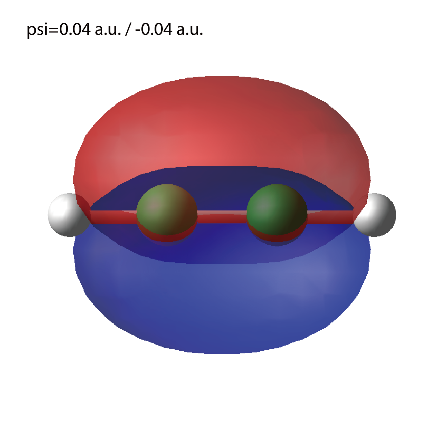
Highest occupied molecular orbital (HOMO)
The output files psi1.cube, psi2.cube, ... are used to create the image.
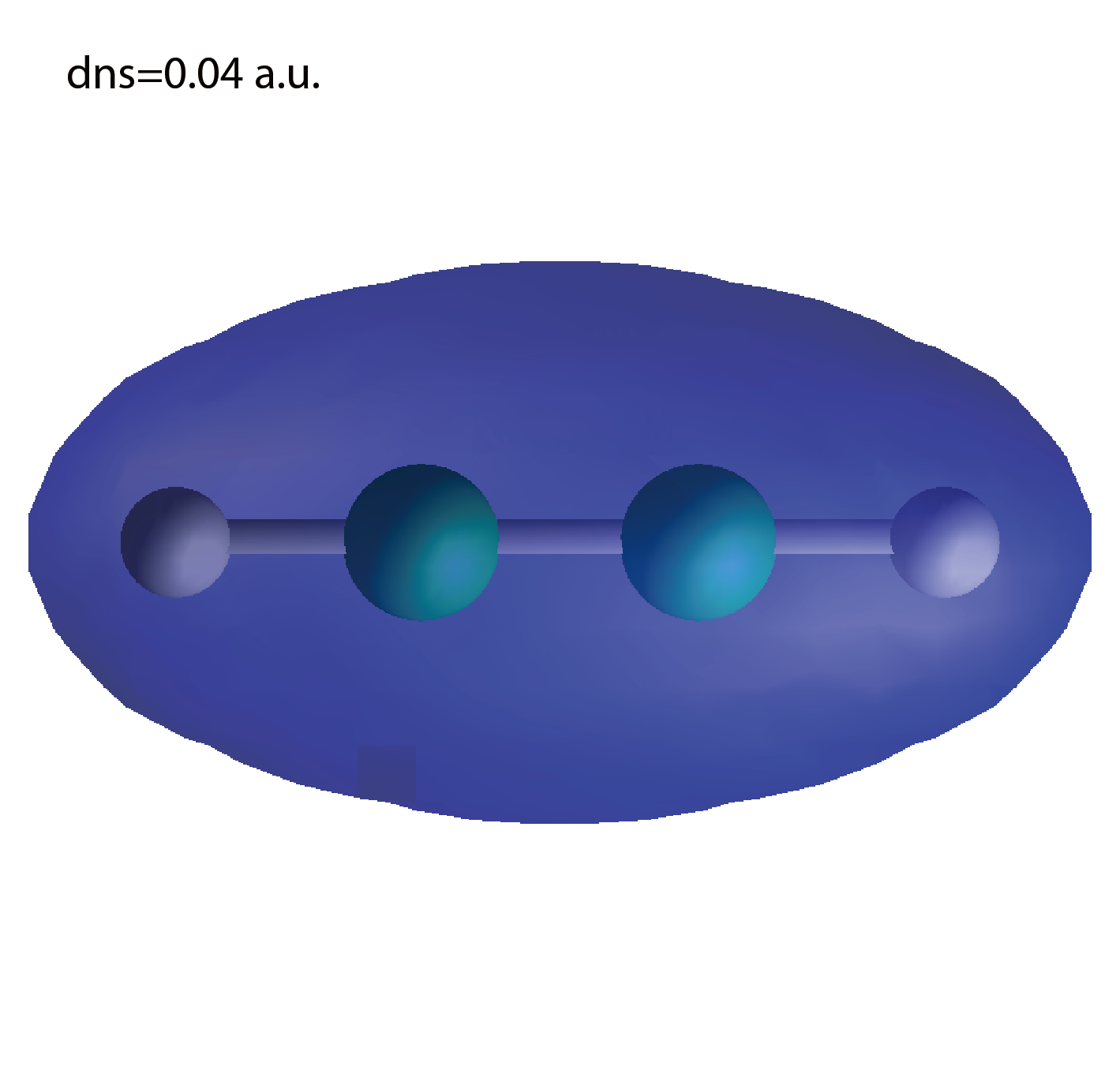
Electron density
The output files dns.cube, ... are used to create the image.
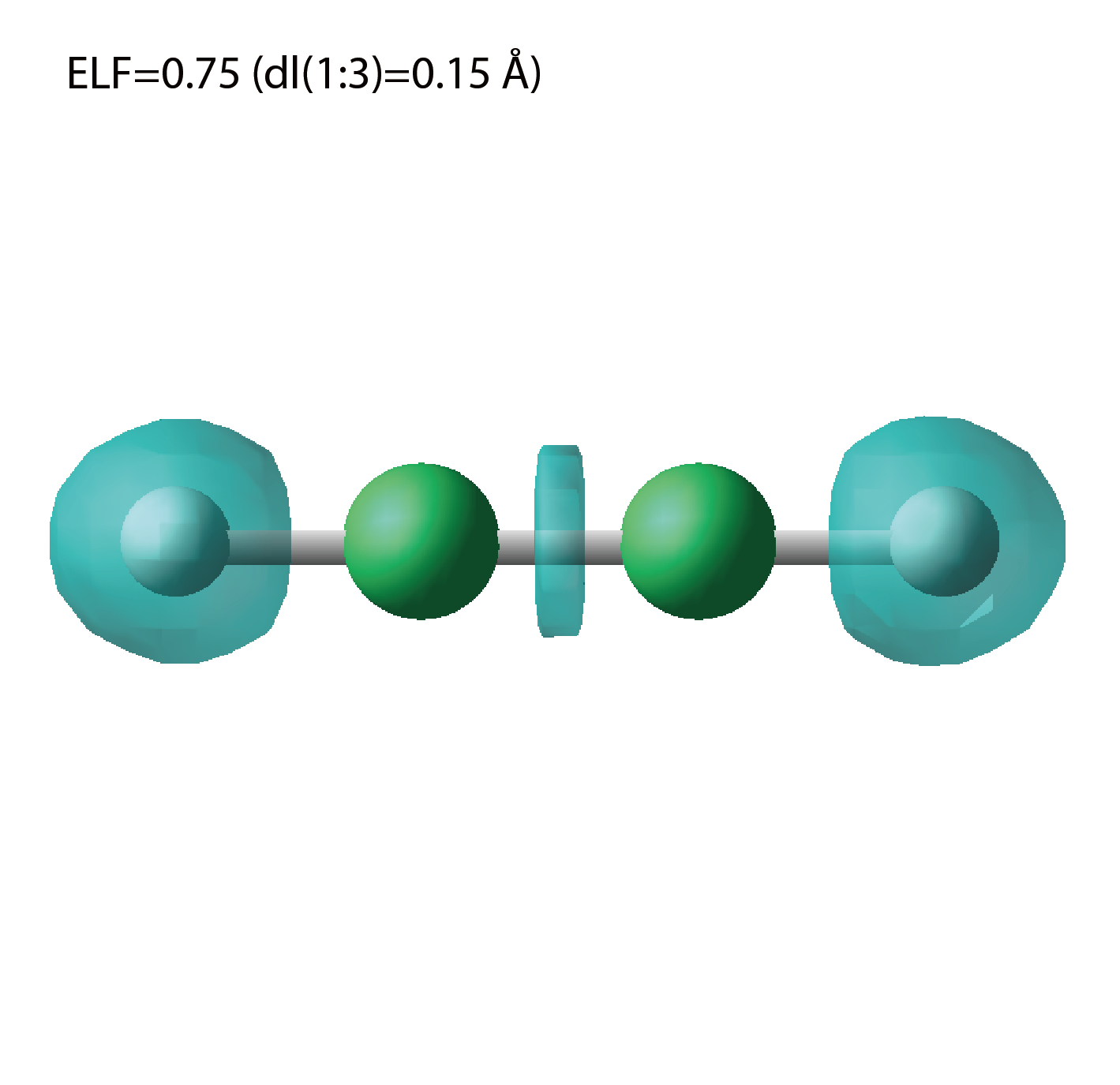
Electron localization function
The output files elf.cube, ... are used to create the image.
Exercise-2: Polarizability and photoabsorption of C2H2 molecule
In this exercise, we learn the linear response calculation in the acetylene (C2H2) molecule, solving the time-dependent Kohn-Sham equation. The linear response calculation provides the polarizability and the oscillator strength distribution of the molecule. This exercise should be carried out after finishing the ground state calculation that was explained in Exercise-1. In the calculation, an impulsive perturbation is applied to all electrons in the C2H2 molecule along the molecular axis which we take z axis. Then a time evolution calculation is carried out without any external fields. During the calculation, the electric dipole moment is monitored. After the time evolution calculation, a time-frequency Fourier transformation is carried out for the electric dipole moment to obtain the frequency-dependent polarizability. The imaginary part of the frequency-dependent polarizability is proportional to the oscillator strength distribution and the photoabsorption cross section.
Input files
To run the code, the input file C2H2_rt_response.inp that contains input keywords and their values for the linear response calculation is required. The binary file C2H2_gs.bin that is created in the ground state calculation and pseudopotential files are also required. The pseudopotential files should be the same as those used in the ground state calculation.
| file name | description |
| C2H2_rt_response.inp | input file that contains input keywords and their values |
| C_rps.dat | pseodupotential file for carbon |
| H_rps.dat | pseudopotential file for hydrogen |
| C2H2_gs.bin | binary file created in the ground state calculation |
In the input file C2H2_rt_response.inp, input keywords are specified. Most of them are mandatory to execute the linear response calculation. This will help you to prepare the input file for other systems that you want to calculate. A complete list of the input keywords that can be used in the input file can be found in the downloaded file SALMON/manual/input_variables.md.
&units
  unit_system='A_eV_fs'
/
&calculation
  calc_mode='RT'
/
&control
  sysname = 'C2H2'
/
&system
  iperiodic = 0
  al = 16d0, 16d0, 16d0
  nstate = 5
  nelem = 2
  natom = 4
  nelec = 10
/
&pseudo
  izatom(1)=6
  izatom(2)=1
  pseudo_file(1)='C_rps.dat'
  pseudo_file(2)='H_rps.dat'
  lmax_ps(1)=1
  lmax_ps(2)=0
  lloc_ps(1)=1
  lloc_ps(2)=0
/
&tgrid
  dt=1.25d-3
  nt=5000
/
&emfield
  ae_shape1 = 'impulse'
  epdir_re1 = 0.d0,0.d0,1.d0
/
&atomic_coor
'C'    0.000000    0.000000    0.599672  1
'H'    0.000000    0.000000    1.662257  2
'C'    0.000000    0.000000   -0.599672  1
'H'    0.000000    0.000000   -1.662257  2
/
We present their explanations below:
Required and recommended variables
&units
Mandatory: none
&units
  unit_system='A_eV_fs'
/
This input keyword specifies the unit system to be used in the input file. If you do not specify it, atomic unit will be used. See &units in Inputs for detail.
&calculation
Mandatory: calc_mode
&calculation
  calc_mode = 'RT'
/
This indicates that the real time (RT) calculation is carried out in the present job. See &calculation in Inputs for detail.
&control
Mandatory: none
&control
  sysname = 'C2H2'
/
'C2H2' defined by sysname = 'C2H2' will be used in the filenames of
output files.
&system
Mandatory: iperiodic, al, nstate, nelem, natom
&system
  iperiodic = 0
  al = 16d0, 16d0, 16d0
  nstate = 5
  nelem = 2
  natom = 4
  nelec = 10
/
These input keywords and their values should be the same as those used in the ground state calculation. See &system in Exercise-1.
&pseudo
Mandatory: pseudo_file, izatom
&pseudo
  izatom(1)=6
  izatom(2)=1
  pseudo_file(1)='C_rps.dat'
  pseudo_file(2)='H_rps.dat'
  lmax_ps(1)=1
  lmax_ps(2)=0
  lloc_ps(1)=1
  lloc_ps(2)=0
/
These input keywords and their values should be the same as those used in the ground state calculation. See &pseudo in Exercise-1.
&tgrid
Mandatory: dt, Nt
&tgrid
  dt=1.25d-3
  nt=5000
/
dt=1.25d-3 specifies the time step of the time evolution
calculation. nt=5000 specifies the number of time steps in the
calculation.
&emfield
Mandatory: ae_shape1
&emfield
  ae_shape1 = 'impulse'
  epdir_re1 = 0.d0,0.d0,1.d0
/
ae_shape1 = 'impulse' indicates that a weak impulse is applied to
all electrons at t=0 epdir_re1(3) specify a unit vector that
indicates the direction of the impulse.
See &emfield in Inputs for details.
&atomic_coor
Mandatory: atomic_coor or atomic_red_coor (it may be provided as a separate file)
&atomic_coor
'C'    0.000000    0.000000    0.599672  1
'H'    0.000000    0.000000    1.662257  2
'C'    0.000000    0.000000   -0.599672  1
'H'    0.000000    0.000000   -1.662257  2
/
Cartesian coordinates of atoms. The first column indicates the element. Next three columns specify Cartesian coordinates of the atoms. The number in the last column labels the element. They must be the same as those in the ground state calculation.
Output files
After the calculation, following output files are created in the directory that you run the code,
| file name | description |
| C2H2_lr.data | polarizability and oscillator strength distribution as functions of energy |
| C2H2_p.data | components of dipole moment as functions of time |
Explanations of the output files are below:
C2H2-p.data
For time steps from 1 to nt,
- 1 column: time
- 2-4 columns: x,y,z components of the dipole moment
- 5 column: total energy of the system
  # time[fs],    dipoleMoment(x,y,z)[A],                        Energy[eV]
  0.12500E-02  0.20197641E-09  0.12143673E-09  0.27407578E-02 -0.33969042E+03
  0.25000E-02 -0.23127543E-09 -0.38283389E-09  0.54651286E-02 -0.33969040E+03
  0.37500E-02 -0.24342401E-08 -0.25180060E-08  0.81587485E-02 -0.33969039E+03
  0.50000E-02 -0.63429482E-08 -0.62611945E-08  0.10810857E-01 -0.33969038E+03
  0.62500E-02 -0.11655064E-07 -0.11294666E-07  0.13413805E-01 -0.33969038E+03

...

  0.62450E+01 -0.21648194E-05 -0.12589717E-05 -0.15217299E-02 -0.33969011E+03
  0.62463E+01 -0.22246530E-05 -0.12919132E-05 -0.14111473E-02 -0.33969011E+03
  0.62475E+01 -0.22836011E-05 -0.13244333E-05 -0.12951690E-02 -0.33969011E+03
  0.62488E+01 -0.23416512E-05 -0.13565206E-05 -0.11738782E-02 -0.33969011E+03
  0.62500E+01 -0.23987916E-05 -0.13881638E-05 -0.10473800E-02 -0.33969011E+03
C2H2_lr.data
For energy steps from 0 to nenergy,
- 1 column: energy
- 2-4 columns: x,y,z components of real part of the polarizability (time-frequency Fourier transformation of the dipole moment)
- 5-7 columns: x,y,z components of imaginary part of the polarizability (time-frequency Fourier transformation of the dipole moment)
- 8-10 columns: x,y,z components of power spectrum of the dipole moment
   # energy[eV], Re[alpha](x,y,z)[A**3], Im[alpha](x,y,z)[A**3], S(x,y,z)[1/eV]
   0.00000E+00  0.90041681E-02  0.42900323E-02  0.47230167E+01  0.00000000E+00  0.00000000E+00  0.00000000E+00  0.00000000E+00  0.00000000E+00  0.00000000E+00
   0.10000E-01  0.89986618E-02  0.42874031E-02  0.47230192E+01  0.25932415E-03  0.12379226E-03  0.18663776E-03  0.15045807E-07  0.71823406E-08  0.10828593E-07
   0.20000E-01  0.89821593E-02  0.42795232E-02  0.47230267E+01  0.51808569E-03  0.24731589E-03  0.37320742E-03  0.60117942E-07  0.28698192E-07  0.43306470E-07
   0.30000E-01  0.89547084E-02  0.42664157E-02  0.47230393E+01  0.77572398E-03  0.37030322E-03  0.55964230E-03  0.13502090E-06  0.64454205E-07  0.97410171E-07
   0.40000E-01  0.89163894E-02  0.42481186E-02  0.47230569E+01  0.10316824E-02  0.49248844E-03  0.74587862E-03  0.23942997E-06  0.11429535E-06  0.17310143E-06
   0.50000E-01  0.88673137E-02  0.42246853E-02  0.47230796E+01  0.12854100E-02  0.61360857E-03  0.93185683E-03  0.37289297E-06  0.17800571E-06  0.27032843E-06

 ...

0.99601E+01  0.15674984E-03  0.37403402E-04 -0.44437601E+00 -0.10631864E-03 -0.14544171E-03  0.27060202E+01 -0.61438595E-05 -0.84046729E-05  0.15637340E+00
0.99701E+01  0.15448331E-03  0.37400902E-04 -0.14920113E+00 -0.10649714E-03 -0.14698080E-03  0.25947889E+01 -0.61603535E-05 -0.85021406E-05  0.15009620E+00
0.99801E+01  0.15224601E-03  0.37478652E-04  0.14911900E+00 -0.10665066E-03 -0.14847068E-03  0.24965858E+01 -0.61754213E-05 -0.85969375E-05  0.14456047E+00
0.99901E+01  0.15003254E-03  0.37632621E-04  0.45012407E+00 -0.10678183E-03 -0.14990965E-03  0.24115316E+01 -0.61892122E-05 -0.86889561E-05  0.13977547E+00
0.10000E+02  0.14783807E-03  0.37858911E-04  0.75334591E+00 -0.10689373E-03 -0.15129625E-03  0.23397373E+01 -0.62019000E-05 -0.87781030E-05  0.13574993E+00
Exercise-3: Electron dynamics in C2H2 molecule under a pulsed electric field
In this exercise, we learn the calculation of the electron dynamics in the acetylene (C2H2) molecule under a pulsed electric field, solving the time-dependent Kohn-Sham equation. As outputs of the calculation, such quantities as the total energy and the electric dipole moment of the system as functions of time are calculated. This tutorial should be carried out after finishing the ground state calculation that was explained in Exercise-1. In the calculation, a pulsed electric field that has cos^2 envelope shape is applied. The parameters that characterize the pulsed field such as magnitude, frequency, polarization direction, and carrier envelope phase are specified in the input file.
Input files
To run the code, following files are used. The C2H2_gs.bin file is created in the ground state calculation. Pseudopotential files are already used in the ground state calculation. Therefore, C2H2_rt_pulse.inp that specifies input keywords and their values for the pulsed electric field calculation is the only file that the users need to prepare.
| file name | description |
| C2H2_rt_pulse.inp | input file that contain input keywords and their values. |
| C_rps.dat | pseodupotential file for Carbon |
| H_rps.dat | pseudopotential file for Hydrogen |
| C2H2_gs.bin | binary file created in the ground state calculation |
In the input file C2H2_rt_pulse.inp, input keywords are specified. Most of them are mandatory to execute the calculation of electron dynamics induced by a pulsed electric field. This will help you to prepare the input file for other systems and other pulsed electric fields that you want to calculate. A complete list of the input keywords that can be used in the input file can be found in the downloaded file SALMON/manual/input_variables.md.
&units
  unit_system='A_eV_fs'
/
&calculation
  calc_mode='RT'
/
&control
  sysname = 'C2H2'
/
&system
  iperiodic = 0
  al = 16d0, 16d0, 16d0
  nstate = 5
  nelem = 2
  natom = 4
  nelec = 10
/
&pseudo
  izatom(1)=6
  izatom(2)=1
  pseudo_file(1)='C_rps.dat'
  pseudo_file(2)='H_rps.dat'
  lmax_ps(1)=1
  lmax_ps(2)=0
  lloc_ps(1)=1
  lloc_ps(2)=0
/
&tgrid
  dt=1.25d-3
  nt=4800
/
&emfield
  ae_shape1 = 'Ecos2'
  epdir_re1 = 0.d0,0.d0,1.d0
  rlaser_int_wcm2_1 = 1.d8
  omega1=9.28d0
  pulse_tw1=6.d0
  phi_cep1=0.75d0
/
&atomic_coor
'C'    0.000000    0.000000    0.599672  1
'H'    0.000000    0.000000    1.662257  2
'C'    0.000000    0.000000   -0.599672  1
'H'    0.000000    0.000000   -1.662257  2
/
We present explanations of the input keywords that appear in the input file below:
required and recommended variables
&units
Mandatory: none
&units
  unit_system='A_eV_fs'
/
This input keyword specifies the unit system to be used in the input file. If you do not specify it, atomic unit will be used. See &units in Inputs for detail.
&calculation
Mandatory: calc_mode
&calculation
  calc_mode = 'RT'
/
This indicates that the real time (RT) calculation is carried out in the present job. See &calculation in Inputs for detail.
&control
Mandatory: none
&control
  sysname = 'C2H2'
/
'C2H2' defined by sysname = 'C2H2' will be used in the filenames of
output files.
&system
Mandatory: iperiodic, al, nstate, nelem, natom
&system
  iperiodic = 0
  al = 16d0, 16d0, 16d0
  nstate = 5
  nelem = 2
  natom = 4
  nelec = 10
/
These input keywords and their values should be the same as those used in the ground state calculation. See &system in Exercise-1.
&pseudo
Mandatory: pseudo_file, izatom
&pseudo
  izatom(1)=6
  izatom(2)=1
  pseudo_file(1)='C_rps.dat'
  pseudo_file(2)='H_rps.dat'
  lmax_ps(1)=1
  lmax_ps(2)=0
  lloc_ps(1)=1
  lloc_ps(2)=0
/
These input keywords and their values should be the same as those used in the ground state calculation. See &pseudo in Exercise-1.
&tgrid
Mandatory: dt, Nt
&tgrid
  dt=1.25d-3
  nt=4800
/
dt=1.25d-3 specifies the time step of the time evolution
calculation. Nt=4800 specifies the number of time steps in the
calculation.
&emfield
Mandatory: ae_shape1, epdir_re1, {rlaser_int1 or amplitude1}, omega1, pulse_tw1, phi_cep1
&emfield
  ae_shape1 = 'Ecos2'
  epdir_re1 = 0.d0,0.d0,1.d0
  rlaser_int_wcm2_1 = 1.d8
  omega1=9.28d0
  pulse_tw1=6.d0
  phi_cep1=0.75d0
/
ae_shape1 = 'Ecos2' indicates that the envelope of the pulsed
electric field has a cos^2 shape.
epdir_re1 = 0.d0,0.d0,1.d0 specifies the real part of the unit
polarization vector of the pulsed electric field. Using the real
polarization vector, it describes a linearly polarized pulse.
laser_int_wcm2_1 = 1.d8 specifies the maximum intensity of the
applied electric field in unit of W/cm^2.
omega1=9.26d0 specifies the average photon energy (frequency
multiplied with hbar).
pulse_tw1=6.d0 specifies the pulse duration. Note that it is not the
FWHM but a full duration of the cos^2 envelope.
phi_cep1=0.75d0 specifies the carrier envelope phase of the pulse.
As noted above, 'phi_cep1' must be 0.75 (or 0.25) if one employs 'Ecos2'
pulse shape, since otherwise the time integral of the electric field
does not vanish.
See &emfield in Inputs for details.
&atomic_coor
Mandatory: atomic_coor or atomic_red_coor (it may be provided as a separate file)
&atomic_coor
'C'    0.000000    0.000000    0.599672  1
'H'    0.000000    0.000000    1.662257  2
'C'    0.000000    0.000000   -0.599672  1
'H'    0.000000    0.000000   -1.662257  2
/
Cartesian coordinates of atoms. The first column indicates the element. Next three columns specify Cartesian coordinates of the atoms. The number in the last column labels the element. They must be the same as those in the ground state calculation.
Output files
After the calculation, following output files are created in the directory that you run the code,
| file name | description |
| C2H2_p.data | components of the electric dipole moment as functions of time |
| C2H2_ps.data | power spectrum that is obtained by a time-frequency Fourier transformation of the electric dipole moment |
Explanations of the files are described below:
C2H2_p.data
For time steps from 1 to nt,
- 1 column: time
- 2-4 columns: x,y,z components of the dipole moment
- 5 column: total energy of the system
  # time[fs],    dipoleMoment(x,y,z)[A],                        Energy[eV]
  0.12500E-02  0.18257556E-09  0.11097584E-09  0.48217422E-09 -0.33970414E+03
  0.25000E-02  0.91251666E-09  0.54016872E-09  0.19424475E-08 -0.33970414E+03
  0.37500E-02  0.24945802E-08  0.14520397E-08  0.43921301E-08 -0.33970414E+03
  0.50000E-02  0.50230110E-08  0.29055651E-08  0.78162260E-08 -0.33970414E+03
  0.62500E-02  0.83018473E-08  0.48072377E-08  0.12178890E-07 -0.33970413E+03

...

  0.59950E+01  0.10101410E-04  0.55756362E-05  0.32250943E-03 -0.33970394E+03
  0.59963E+01  0.10109316E-04  0.55775491E-05  0.38471398E-03 -0.33970394E+03
  0.59975E+01  0.10115053E-04  0.55780512E-05  0.44680913E-03 -0.33970394E+03
  0.59988E+01  0.10118632E-04  0.55771582E-05  0.50877609E-03 -0.33970394E+03
  0.60000E+01  0.10120064E-04  0.55748807E-05  0.57059604E-03 -0.33970394E+03
C2H2_ps.data
For energy steps from 0 to nenergy,
- 1 column: energy
- 2-4 columns: x,y,z components of the real part of the time-frequency Fourier transformation of the dipole moment
- 5-7 columns: x,y,z components of imaginary part of the time-frequency Fourier transformation of the dipole moment
- 8-10 columns: x,y,z components of power spectrum of the dipole moment
  # energy[eV], Re[alpha](x,y,z)[A*fs], Im[alpha](x,y,z)[A*fs], I(x,y,z)[A**2*fs**2]
   0.00000E+00  0.12836214E-01  0.60771681E-02 -0.28240863E-02  0.00000000E+00  0.00000000E+00  0.00000000E+00  0.16476838E-03  0.36931972E-04  0.79754632E-05
   0.10000E-01  0.12829079E-01  0.60737829E-02 -0.28241953E-02  0.35253318E-03  0.16719128E-03 -0.41437502E-04  0.16470954E-03  0.36918792E-04  0.79777964E-05
   0.20000E-01  0.12807693E-01  0.60636364E-02 -0.28245142E-02  0.70436985E-03  0.33405211E-03 -0.83009748E-04  0.16453313E-03  0.36879277E-04  0.79847710E-05
   0.30000E-01  0.12772113E-01  0.60467557E-02 -0.28250177E-02  0.10548158E-02  0.50025311E-03 -0.12484976E-03  0.16423951E-03  0.36813507E-04  0.79963126E-05
   0.40000E-01  0.12722434E-01  0.60231857E-02 -0.28256644E-02  0.14031812E-02  0.66546701E-03 -0.16708711E-03  0.16382925E-03  0.36721612E-04  0.80122973E-05
   0.50000E-01  0.12658789E-01  0.59929893E-02 -0.28263966E-02  0.17487830E-02  0.82936975E-03 -0.20984627E-03  0.16330319E-03  0.36603775E-04  0.80325532E-05

 ...

0.99601E+01  0.38757368E-03  0.19783358E-03  0.11087376E+01 -0.27465428E-03 -0.29515838E-03  0.10183658E+01  0.22564833E-06  0.12625659E-06  0.22663679E+01
0.99701E+01  0.38446279E-03  0.19754997E-03  0.10416956E+01 -0.27241140E-03 -0.29512921E-03  0.10381647E+01  0.22201960E-06  0.12612724E-06  0.21629157E+01
0.99801E+01  0.38136406E-03  0.19733388E-03  0.97519659E+00 -0.27017795E-03 -0.29508231E-03  0.10542348E+01  0.21843467E-06  0.12601423E-06  0.20624194E+01
0.99901E+01  0.37827032E-03  0.19718146E-03  0.90943725E+00 -0.26795413E-03 -0.29501502E-03  0.10666811E+01  0.21488785E-06  0.12591439E-06  0.19648847E+01
0.10000E+02  0.37517469E-03  0.19708886E-03  0.84460457E+00 -0.26574105E-03 -0.29492512E-03  0.10756186E+01  0.21137435E-06  0.12582485E-06  0.18703122E+01
Crystalline silicon (periodic solids)
Exercise-4: Dielectric function of crystalline silicon
In this exercise, we learn the linear response calculation of the crystalline silicon of a diamond structure. Calculation is done in a cubic unit cell that contains eight silicon atoms. Since the ground state calculation costs much less computational time than the time evolution calculation, both calculations are successively executed. After finishing the ground state calculation, an impulsive perturbation is applied to all electrons in the unit cell along z direction. Since the dielectric function is isotropic in the diamond structure, calculated dielectric function should not depend on the direction of the perturbation. During the time evolution, electric current averaged over the unit cell volume is calculated. A time-frequency Fourier transformation of the electric current gives us a frequency-dependent conductivity. The dielectric function may be obtained from the conductivity using a standard relation.
Input files
To run the code, following files are used:
| file name | description |
| Si_gs_rt_response.inp | input file that contain input keywords and their values. |
| Si_rps.dat | pseodupotential file of silicon |
In the input file Si_gs_rt_response.inp, input keywords are specified. Most of them are mandatory to execute the calculation. This will help you to prepare the input file for other systems that you want to calculate. A complete list of the input keywords that can be used in the input file can be found in the downloaded file SALMON/manual/input_variables.md.
&calculation
  calc_mode = 'GS_RT'
/
&control
  sysname = 'Si'
/
&units
  unit_system = 'a.u.'
/
&system
  iperiodic = 3
  al = 10.26d0, 10.26d0, 10.26d0
  nstate = 32
  nelec = 32
  nelem = 1
  natom = 8
/
&pseudo
  izatom(1) = 14
  pseudo_file(1) = './Si_rps.dat'
  lloc_ps(1) = 2
/
&functional
  xc = 'PZ'
/
&rgrid
  num_rgrid = 12, 12, 12
/
&kgrid
  num_kgrid = 4, 4, 4
/
&tgrid
  nt = 3000
  dt = 0.16
/
&propagation
  propagator = 'etrs'
/
&scf
  ncg = 5
  nscf = 120
/
&emfield
  trans_longi = 'tr'
  ae_shape1 = 'impulse'
  epdir_re1 = 0., 0., 1.
/
&analysis
  nenergy = 1000
  de = 0.001
/
&atomic_red_coor
  'Si'       .0      .0      .0      1
  'Si'       .25     .25     .25     1
  'Si'       .5      .0      .5      1
  'Si'       .0      .5      .5      1
  'Si'       .5      .5      .0      1
  'Si'       .75     .25     .75     1
  'Si'       .25     .75     .75     1
  'Si'       .75     .75     .25     1
/
We present explanations of the input keywords that appear in the input file below:
&calculation
Mandatory: calc_mode
&calculation
  calc_mode = 'GS_RT'
/
This indicates that the ground state (GS) and the real time (RT) calculations are carried out sequentially in the present job. See &calculation in Inputs for detail.
&control
Mandatory: none
&control
  sysname = 'Si'
/
'Si' defined by sysname = 'C2H2' will be used in the filenames of
output files.
&system
Mandatory: periodic, al, state, nelem, natom
&system
  iperiodic = 3
  al = 10.26d0,10.26d0,10.26d0
  nstate = 32
  nelec = 32
  nelem = 1
  natom = 8
/
iperiodic = 3 indicates that three dimensional periodic boundary
condition (bulk crystal) is assumed. al = 10.26d0, 10.26d0, 10.26d0
specifies the lattice constans of the unit cell. nstate = 32
indicates the number of Kohn-Sham orbitals to be solved. nelec = 32
indicate the number of valence electrons in the system. nelem = 1
and natom = 8 indicate the number of elements and the number of
atoms in the system, respectively.
See &system in Inputs for more information.
&pseudo
&pseudo
  izatom(1)=14
  pseudo_file(1) = './Si_rps.dat'
  lloc_ps(1)=2
/
izatom(1) = 14 indicates the atomic number of the element #1.
pseudo_file(1) = 'Si_rps.dat' indicates the pseudopotential filename
of element #1. lloc_ps(1) = 2 indicate the angular momentum of the
pseudopotential that will be treated as local.
&functional
&functional
  xc = 'PZ'
/
This indicates that the adiabatic local density approximation with the Perdew-Zunger functional is used. We note that meta-GGA functionals that reasonably reproduce the band gap of various insulators may also be used in the calculation of periodic systems. See &functional in Inputs for detail.
&rgrid
Mandatory: dl or num_rgrid
&rgrid
  num_rgrid = 12,12,12
/
num_rgrid=12,12,12 specifies the number of the grids for each
Cartesian direction. See &rgrid in Inputs for more information.
&kgrid
Mandatory: none
This input keyword provides grid spacing of k-space for periodic systems.
&kgrid
  num_kgrid = 4,4,4
/
&tgrid
&tgrid
 nt=3000
 dt=0.16
/
dt=0.16 specifies the time step of the time evolution calculation.
nt=3000 specifies the number of time steps in the calculation.
&propagation
&propagation
  propagator='etrs'
/
propagator = 'etrs' indicates the use of enforced time-reversal
symmetry propagator.
See &propagation in Inputs for more information.
&scf
Mandatory: nscf
This input keywords specify parameters related to the self-consistent field calculation.
&scf
  ncg = 5
  nscf = 120
/
ncg = 5 is the number of conjugate-gradient iterations in solving
the Kohn-Sham equation. Usually this value should be 4 or 5.
nscf = 120 is the number of scf iterations.
&emfield
Mandatory:ae_shape1
&emfield
  trans_longi = 'tr'
  ae_shape1 = 'impulse'
  epdir_re1 = 0.,0.,1.
/
as_shape1 = 'impulse' indicates that a weak impulsive field is
applied to all electrons at t=0
epdir_re1(3) specify a unit vector that indicates the direction of
the impulse.
trans_longi = 'tr' specifies the treatment of the polarization in
the time evolution calculation, transverse for 'tr' and longitudinal for
'lo'.
See &emfield in Inputs for detail.
&analysis
&analysis
 nenergy=1000
 de=0.001
/
nenergy=1000 specifies the number of energy steps, and de=0.001
specifies the energy spacing in the time-frequency Fourier
transformation.
&atomic_red_coor
Mandatory: atomic_coor or atomic_red_coor (they may be provided as a separate file)
&atomic_red_coor
 'Si'    .0      .0      .0      1
 'Si'    .25    .25    .25    1
 'Si'    .5      .0      .5      1
 'Si'    .0      .5      .5      1
 'Si'    .5      .5      .0      1
 'Si'    .75    .25   .75     1
 'Si'    .25    .75   .75     1
 'Si'    .75    .75   .25     1
/
Cartesian coordinates of atoms are specified in a reduced coordinate system. First column indicates the element, next three columns specify reduced Cartesian coordinates of the atoms, and the last column labels the element.
Output files
After the calculation, following output files are created in the directory that you run the code,
| file name | description |
| Si_gs_info.data | information of ground state calculation |
| Si_eigen.data | energy eigenvalues of orbitals |
| Si_k.data | information on k-points |
| Si_rt.data | electric field, vector potential, and current as functions of time |
| Si_force.data | force acting on atoms |
| Si_lr.data | Fourier spectra of the dielectric functions |
| Si_gs_rt_response.out | standard output file |
Explanations of the output files are described below:
Si_gs_info.data
Results of the ground state as well as input parameters are provided.
 #---------------------------------------------------------
 #grid information-----------------------------------------
 #aL =   10.2600000000000        10.2600000000000        10.2600000000000
 #al(1),al(2),al(3) =   10.2600000000000        10.2600000000000
   10.2600000000000
 #aLx,aLy,aLz =   10.2600000000000        10.2600000000000
   10.2600000000000
 #bLx,bLy,bLz =  0.612396228769940       0.612396228769940
  0.612396228769940
 #Nd =           4
 #NLx,NLy,NLz=          12          12          12
 #NL =        1728
 #Hx,Hy,Hz =  0.855000000000000       0.855000000000000
  0.855000000000000
 #(pi/max(Hx,Hy,Hz))**2 =   13.5010490764192
 #(pi/Hx)**2+(pi/Hy)**2+(pi/Hz)**2 =   40.5031472292576
 #Hxyz =  0.625026375000000
 #NKx,NKy,NKz=           4           4           4
 #NKxyz =          64
 #Sym=           1
 #NK =          64
 #NEwald, aEwald =           4  0.500000000000000
 #---------------------------------------------------------
 #GS calc. option------------------------------------------
 #FSset_option =n
 #Ncg=           5
 #Nmemory_MB,alpha_MB =           8  0.750000000000000
 #NFSset_start,NFSset_every =          75          25
 #Nscf=         120
 #Nscf_conv=         120
 #NI,NE=           8           1
 #Zatom=          14
 #Lref=           2
 #i,Kion(ia)(Rion(j,a),j=1,3)
 #           1           1
 #  0.000000000000000E+000  0.000000000000000E+000  0.000000000000000E+000
 #           2           1
 #   2.56500000000000        2.56500000000000        2.56500000000000
 #           3           1
 #   5.13000000000000       0.000000000000000E+000   5.13000000000000
 #           4           1
 #  0.000000000000000E+000   5.13000000000000        5.13000000000000
 #           5           1
 #   5.13000000000000        5.13000000000000       0.000000000000000E+000
 #           6           1
 #   7.69500000000000        2.56500000000000        7.69500000000000
 #           7           1
 #   2.56500000000000        7.69500000000000        7.69500000000000
 #           8           1
 #   7.69500000000000        7.69500000000000        2.56500000000000
 #---------------------------------------------------------
 #GS information-------------------------------------------
 #NB,Nelec=          32          32
 #Eall =  -31.2658878806236
 #ddns(iter = Nscf_conv)  2.798849279746559E-010
 #ddns_abs_1e(iter = Nscf_conv)  2.364732236264119E-010
 #esp_var_ave(iter = Nscf_conv)  1.196976937606010E-009
 #esp_var_max(iter = Nscf_conv)  4.031276129792963E-009
 #NBoccmax is           16
 #---------------------------------------------------------
 #band information-----------------------------------------
 #Bottom of VB -0.194802063980608
 #Top of VB  0.216731478175047
 #Bottom of CB  0.255681914576368
 #Top of CB  0.533214678236198
 #Fundamental gap  3.895043640132098E-002
 #Fundamental gap[eV]   1.05990369517819
 #BG between same k-point  3.895043648321342E-002
 #BG between same k-point[eV]   1.05990369740661
 #Physicaly upper bound of CB for DOS  0.454100922291231
 #Physicaly upper bound of CB for eps(omega)  0.609752486428134
 #---------------------------------------------------------
 #iter     total-energy          ddns/nelec         esp_var_ave         esp_var_max
     1   -0.2059780903E+02    0.5134199377E+00    0.1332473220E-01    0.1986049398E-01
     2   -0.2600097163E+02    0.3186108570E+00    0.1526707771E-01    0.2520724900E-01
     3   -0.2866336088E+02    0.1363849859E+00    0.6359704895E-02    0.1247448390E-01
     4   -0.3006244467E+02    0.1245614607E+00    0.5868323970E-02    0.1942874074E-01
     5   -0.3096872596E+02    0.7495214064E-01    0.2566344769E-02    0.1102001262E-01

...

   115   -0.3126588788E+02    0.1355175468E-09    0.1208579378E-08    0.4031265522E-08
   116   -0.3126588788E+02    0.1452261250E-09    0.1204317051E-08    0.4031272647E-08
   117   -0.3126588788E+02    0.1419175726E-09    0.1198067051E-08    0.4031255783E-08
   118   -0.3126588788E+02    0.1686476198E-09    0.1198945057E-08    0.4031251395E-08
   119   -0.3126588788E+02    0.2159059511E-09    0.1200809994E-08    0.4666412657E-08
   120   -0.3126588788E+02    0.2364732236E-09    0.1196976938E-08    0.4031276130E-08
Si_eigen.data
Orbital energies in the ground state calculation.
# Ground state eigenenergies
# ik: k-point index
# ib: Band index
# energy: Eigenenergy
# occup: Occupation
# 1:ik[none] 2:ib[none] 3:energy[a.u.] 4:occup[none]
     1      1 -1.38676447625070E-001  2.00000000000000E+000
     1      2 -1.10783431105032E-001  2.00000000000000E+000
     1      3 -1.10783428207470E-001  2.00000000000000E+000
     1      4 -1.10783427594037E-001  2.00000000000000E+000
     1      5 -1.57456296850928E-002  2.00000000000000E+000

...

    64     28  3.68051950109468E-001  0.00000000000000E+000
    64     29  4.91528586750629E-001  0.00000000000000E+000
    64     30  4.91528587785578E-001  0.00000000000000E+000
    64     31  4.91528588058071E-001  0.00000000000000E+000
    64     32  5.14831956233275E-001  0.00000000000000E+000
Si_k.data
Information on k-points.
# k-point distribution
# ik: k-point index
# kx,ky,kz: Reduced coordinate of k-points
# wk: Weight of k-point
# 1:ik[none] 2:kx[none] 3:ky[none] 4:kz[none] 5:wk[none]
     1 -3.75000000000000E-001 -3.75000000000000E-001 -3.75000000000000E-001  1.00000000000000E+000
     2 -3.75000000000000E-001 -3.75000000000000E-001 -1.25000000000000E-001  1.00000000000000E+000
     3 -3.75000000000000E-001 -3.75000000000000E-001  1.25000000000000E-001  1.00000000000000E+000
     4 -3.75000000000000E-001 -3.75000000000000E-001  3.75000000000000E-001  1.00000000000000E+000
     5 -3.75000000000000E-001 -1.25000000000000E-001 -3.75000000000000E-001  1.00000000000000E+000

...

    60  3.75000000000000E-001  1.25000000000000E-001  3.75000000000000E-001  1.00000000000000E+000
    61  3.75000000000000E-001  3.75000000000000E-001 -3.75000000000000E-001  1.00000000000000E+000
    62  3.75000000000000E-001  3.75000000000000E-001 -1.25000000000000E-001  1.00000000000000E+000
    63  3.75000000000000E-001  3.75000000000000E-001  1.25000000000000E-001  1.00000000000000E+000
    64  3.75000000000000E-001  3.75000000000000E-001  3.75000000000000E-001  1.00000000000000E+000
Si_rt.data
Results of time evolution calculation. Ac_ext_x,y,z are applied vector
potential. For transverse calculation specified by trans_longi = 'tr',
Ac_tot_x,y,z are equal to Ac_ext_x,y,z. For longitudinal calculation
specified by trans_longi = 'lo', Ac_tot_x,y,z are the sum of
Ac_ext_x,y,z and the induced polarization. The same relation holds for
electric fields of E_ext_x,y,z and E_tot_x,y,z. Jm_x,y,z are
macroscopic current. Eall and Eall-Eall0 are total energy and
electronic excitation energy, respectively. ''Tion' is the kinetic
energy of atoms. Temperature_ion is the temperature estimated from the
atomic motion.
# Real time calculation
# Ac_ext: External vector potential field
# E_ext: External electric field
# Ac_tot: Total vector potential field
# E_tot: Total electric field
# Jm: Matter current density
# Eall: Total energy
# Eall0: Initial energy
# Tion: Kinetic energy of ions
# 1:Time[a.u.] 2:Ac_ext_x[a.u.] 3:Ac_ext_y[a.u.] 4:Ac_ext_z[a.u.] 5:E_ext_x[a.u.] 6:E_ext_y[a.u.] 7:E_ext_z[a.u.] 8:Ac_tot_x[a.u.] 9:Ac_tot_y[a.u.] 10:Ac_tot_z[a.u.] 11:E_tot_x[a.u.] 12:E_tot_y[a.u.] 13:E_tot_z[a.u.] 14:Jm_x[a.u.] 15:Jm_y[a.u.] 16:Jm_z[a.u.] 17:Eall[a.u.] 18:Eall-Eall0[a.u.] 19:Tion[a.u.] 20:Temperature_ion[K]
      0.00000000  0.00000000000000E+000  0.00000000000000E+000  1.00000000000000E-002  0.00000000000000E+000  0.00000000000000E+000  0.00000000000000E+000  0.00000000000000E+000  0.00000000000000E+000  1.00000000000000E-002  0.00000000000000E+000  0.00000000000000E+000  0.00000000000000E+000 -8.65860214541267E-013  1.04880923197437E-012  2.79610491078699E-004 -3.12643773655041E+001  1.51051511945255E-003  0.00000000000000E+000  0.00000000000000E+000
      0.16000000  0.00000000000000E+000  0.00000000000000E+000  1.00000000000000E-002  0.00000000000000E+000  0.00000000000000E+000  0.00000000000000E+000  0.00000000000000E+000  0.00000000000000E+000  1.00000000000000E-002  0.00000000000000E+000  0.00000000000000E+000  0.00000000000000E+000 -7.80220609595942E-013  1.25669598865900E-012  2.77640461612200E-004 -3.12643780708603E+001  1.50980976327020E-003  0.00000000000000E+000  0.00000000000000E+000
      0.32000000  0.00000000000000E+000  0.00000000000000E+000  1.00000000000000E-002  0.00000000000000E+000  0.00000000000000E+000  0.00000000000000E+000  0.00000000000000E+000  0.00000000000000E+000  1.00000000000000E-002  0.00000000000000E+000  0.00000000000000E+000  0.00000000000000E+000 -6.65469342838961E-013  1.44166600383436E-012  2.72256619397668E-004 -3.12643780794812E+001  1.50980114240440E-003  0.00000000000000E+000  0.00000000000000E+000
      0.48000000  0.00000000000000E+000  0.00000000000000E+000  1.00000000000000E-002  0.00000000000000E+000  0.00000000000000E+000  0.00000000000000E+000  0.00000000000000E+000  0.00000000000000E+000  1.00000000000000E-002  0.00000000000000E+000  0.00000000000000E+000  0.00000000000000E+000 -5.07694047189471E-013  1.65330407801294E-012  2.65100129464106E-004 -3.12643780384343E+001  1.50984218925032E-003  0.00000000000000E+000  0.00000000000000E+000
      0.64000000  0.00000000000000E+000  0.00000000000000E+000  1.00000000000000E-002  0.00000000000000E+000  0.00000000000000E+000  0.00000000000000E+000  0.00000000000000E+000  0.00000000000000E+000  1.00000000000000E-002  0.00000000000000E+000  0.00000000000000E+000  0.00000000000000E+000 -3.21400178809861E-013  1.87627749522222E-012  2.57460045574299E-004 -3.12643779799564E+001  1.50990066720169E-003  0.00000000000000E+000  0.00000000000000E+000

...

    479.36000000  0.00000000000000E+000  0.00000000000000E+000  1.00000000000000E-002  0.00000000000000E+000  0.00000000000000E+000  0.00000000000000E+000  0.00000000000000E+000  0.00000000000000E+000  1.00000000000000E-002  0.00000000000000E+000  0.00000000000000E+000  0.00000000000000E+000 -7.94263263896610E-013  3.79557494087330E-012 -3.59285386087180E-006 -3.12643819342307E+001  1.50594639281820E-003  0.00000000000000E+000  0.00000000000000E+000
    479.52000000  0.00000000000000E+000  0.00000000000000E+000  1.00000000000000E-002  0.00000000000000E+000  0.00000000000000E+000  0.00000000000000E+000  0.00000000000000E+000  0.00000000000000E+000  1.00000000000000E-002  0.00000000000000E+000  0.00000000000000E+000  0.00000000000000E+000 -5.67828280529921E-013  3.78374121551490E-012 -2.90523320634650E-006 -3.12643819351033E+001  1.50594552028593E-003  0.00000000000000E+000  0.00000000000000E+000
    479.68000000  0.00000000000000E+000  0.00000000000000E+000  1.00000000000000E-002  0.00000000000000E+000  0.00000000000000E+000  0.00000000000000E+000  0.00000000000000E+000  0.00000000000000E+000  1.00000000000000E-002  0.00000000000000E+000  0.00000000000000E+000  0.00000000000000E+000 -3.61839313869103E-013  3.74173331529800E-012 -2.24958911411780E-006 -3.12643819359872E+001  1.50594463632103E-003  0.00000000000000E+000  0.00000000000000E+000
    479.84000000  0.00000000000000E+000  0.00000000000000E+000  1.00000000000000E-002  0.00000000000000E+000  0.00000000000000E+000  0.00000000000000E+000  0.00000000000000E+000  0.00000000000000E+000  1.00000000000000E-002  0.00000000000000E+000  0.00000000000000E+000  0.00000000000000E+000 -1.73847971134404E-013  3.66573716775167E-012 -1.63591499831827E-006 -3.12643819368722E+001  1.50594375133295E-003  0.00000000000000E+000  0.00000000000000E+000
    480.00000000  0.00000000000000E+000  0.00000000000000E+000  1.00000000000000E-002  0.00000000000000E+000  0.00000000000000E+000  0.00000000000000E+000  0.00000000000000E+000  0.00000000000000E+000  1.00000000000000E-002  0.00000000000000E+000  0.00000000000000E+000  0.00000000000000E+000  3.16688678319438E-016  3.55459629253500E-012 -1.06271326454723E-006 -3.12643819377811E+001  1.50594284247063E-003  0.00000000000000E+000  0.00000000000000E+000
Si_force.data
Force acting on each atom during time evolution.
# Force calculatio
# force: Force
# time[a.u.] force[a.u.]
    0.000000E+000  -0.663815E-008   0.381467E-008   0.178186E-002   0.280496E-008   0.236613E-009   0.178187E-002   0.190620E-008   0.346038E-008   0.178186E-002  -0.255965E-008   0.162582E-008   0.178187E-002  -0.713246E-009  -0.607621E-008   0.178187E-002  -0.124821E-008   0.434748E-008   0.178187E-002  -0.932639E-008  -0.112168E-007   0.178187E-002  -0.505708E-008  -0.289586E-008   0.178187E-002
    0.160000E+001  -0.131290E-008   0.165516E-008   0.339940E-002  -0.941496E-009  -0.767670E-009   0.339940E-002   0.138786E-008   0.172143E-008   0.339940E-002  -0.451825E-009  -0.106362E-008   0.339940E-002   0.298232E-009   0.383164E-009   0.339940E-002  -0.296521E-009  -0.195556E-008   0.339940E-002   0.348404E-009  -0.849494E-009   0.339940E-002  -0.297429E-009   0.578589E-009   0.339940E-002
    0.320000E+001   0.615410E-008  -0.278186E-008   0.457711E-002  -0.486320E-008  -0.116861E-008   0.457711E-002  -0.112143E-008  -0.166802E-008   0.457711E-002   0.253122E-008  -0.368112E-008   0.457710E-002   0.935799E-009   0.830658E-008   0.457711E-002   0.621491E-009  -0.804263E-008   0.457710E-002   0.123310E-007   0.130141E-007   0.457711E-002   0.636436E-008   0.330898E-008   0.457710E-002
    0.480000E+001   0.635332E-008  -0.357991E-008   0.446307E-002  -0.388157E-008  -0.157542E-008   0.446307E-002  -0.193530E-008  -0.255271E-008   0.446308E-002   0.230966E-008  -0.227850E-008   0.446306E-002  -0.341100E-009   0.746659E-008   0.446307E-002   0.734950E-009  -0.635113E-008   0.446307E-002   0.943051E-008   0.126831E-007   0.446307E-002   0.494958E-008   0.330406E-008   0.446306E-002
    0.640000E+001   0.407644E-009   0.406484E-010   0.320569E-002   0.134973E-008  -0.648732E-009   0.320569E-002  -0.148635E-009  -0.650159E-009   0.320569E-002  -0.231759E-009   0.163276E-008   0.320569E-002  -0.961535E-009  -0.941812E-009   0.320569E-002   0.847442E-009   0.130553E-008   0.320569E-002  -0.264725E-008  -0.351407E-009   0.320569E-002  -0.141512E-008   0.421806E-009   0.320569E-002

...

    0.473600E+003   0.246506E-009   0.251205E-009  -0.148216E-003  -0.416554E-011   0.779853E-009  -0.148215E-003  -0.115879E-009   0.104374E-008  -0.148217E-003   0.913004E-009  -0.465967E-009  -0.148217E-003   0.176729E-009  -0.270103E-009  -0.148216E-003   0.962326E-009   0.799398E-009  -0.148218E-003   0.220066E-009  -0.152063E-008  -0.148216E-003   0.571304E-009  -0.132336E-008  -0.148217E-003
    0.475200E+003  -0.504521E-009  -0.437234E-010  -0.316399E-003  -0.459509E-009   0.105940E-008  -0.316398E-003   0.105290E-009   0.547364E-009  -0.316401E-003   0.181887E-009  -0.343314E-009  -0.316399E-003  -0.804290E-010  -0.500340E-009  -0.316400E-003   0.372911E-009   0.141733E-008  -0.316401E-003  -0.244574E-009  -0.259207E-008  -0.316400E-003   0.202885E-009  -0.147976E-008  -0.316400E-003
    0.476800E+003  -0.475521E-009  -0.161693E-009  -0.415900E-003  -0.925954E-009   0.240941E-009  -0.415900E-003   0.291237E-009  -0.453400E-009  -0.415902E-003  -0.580783E-009  -0.751060E-010  -0.415900E-003  -0.683807E-009  -0.202391E-010  -0.415902E-003  -0.618227E-011   0.138283E-008  -0.415902E-003  -0.274419E-009  -0.218740E-008  -0.415901E-003   0.175364E-009  -0.657477E-009  -0.415900E-003
    0.478400E+003   0.303920E-009  -0.402101E-009  -0.439830E-003  -0.134116E-008  -0.816066E-009  -0.439830E-003   0.318015E-009  -0.927198E-009  -0.439831E-003  -0.150791E-008  -0.169799E-009  -0.439831E-003  -0.702142E-009   0.881452E-009  -0.439831E-003  -0.618720E-009   0.779075E-009  -0.439831E-003   0.540736E-009   0.352559E-009  -0.439830E-003   0.382572E-009   0.794098E-009  -0.439830E-003
    0.480000E+003   0.957060E-009  -0.635421E-009  -0.336591E-003  -0.873698E-009  -0.134192E-008  -0.336592E-003  -0.660852E-010  -0.282862E-009  -0.336591E-003  -0.156118E-008  -0.398368E-009  -0.336593E-003  -0.480887E-010   0.961042E-009  -0.336592E-003  -0.121634E-008  -0.277887E-009  -0.336591E-003   0.104632E-008   0.244269E-008  -0.336591E-003   0.412975E-009   0.133042E-008  -0.336591E-003
Si_lr_data
In transverse calculation specified by trans_longi = 'tr',
time-frequency Fourier transformation of the macroscopic current gives
the conductivity of the system. Then the dielectric function is
calculated.
# Fourier-transform spectra
# sigma: Conductivity
# eps: Dielectric constant
# 1:Frequency[a.u.] 2:Re(sigma_x)[a.u.] 3:Re(sigma_y)[a.u.] 4:Re(sigma_z)[a.u.] 5:Im(sigma_x)[a.u.] 6:Im(sigma_y)[a.u.] 7:Im(sigma_z)[a.u.] 8:Re(eps_x)[none] 9:Re(eps_y)[none] 10:Re(eps_z)[none] 11:Im(eps_x)[none] 12:Im(eps_y)[none] 13:Im(eps_z)[none]
      0.00100000 -1.03308449903699E-010 -2.55685769383253E-011  3.36356888185559E-005  9.38757700305135E-010  2.38405472055867E-010 -1.31839196070590E-003 -1.17967771791178E-005 -2.99589151834528E-006  1.75674019932220E+001 -1.29821226908484E-006 -3.21304213888753E-007  4.22678531563230E-001
      0.00200000 -4.05463997396279E-010 -1.00459000515141E-010  1.32405016849080E-004  1.82449482725124E-009  4.64061580393162E-010 -2.62118275831395E-003 -1.14636390916102E-005 -2.91578490355285E-006  1.74693769944707E+001 -2.54760543103060E-006 -6.31202516010683E-007  8.31925256463007E-001
      0.00300000 -8.83952914849078E-010 -2.19401192737277E-010  2.90077713140610E-004  2.60896580505206E-009  6.65304400028214E-010 -3.89397682658909E-003 -1.09284104088247E-005 -2.78682055403947E-006  1.73110519888816E+001 -3.70269331121220E-006 -9.19025567056355E-007  1.21507468343022E+000
      0.00400000 -1.50380858485809E-009 -3.74177620806077E-010  4.96861248105049E-004  3.25293966934794E-009  8.32525470173577E-010 -5.12467699872510E-003 -1.02194113677943E-005 -2.61545590102370E-006  1.70996476112154E+001 -4.72435400259545E-006 -1.17551366466208E-006  1.56093564690028E+000
      0.00500000 -2.22112273174113E-009 -5.54404046892706E-010  7.40224957578435E-004  3.72943718693087E-009  9.58925096932178E-010 -6.30436402916416E-003 -9.37309797478928E-006 -2.41004163189201E-006  1.68445949756623E+001 -5.58229028540739E-006 -1.39336934467086E-006  1.86038823098578E+000

...


      0.99600000 -2.76735852669967E-009 -1.50791378263185E-009  4.18549443295463E-003 -3.48281730295103E-010 -2.38950132823120E-011  2.58042637047465E-002  4.39421415772947E-009  3.01479510783703E-010  6.74431785999496E-001 -3.49153141258183E-008 -1.90251038625021E-008  5.28077050691215E-002
      0.99700000 -2.79907084112808E-009 -1.43228946145853E-009  4.21502473100264E-003 -4.64190825344567E-010 -1.65916319932293E-010  2.58406831005378E-002  5.85074618562197E-009  2.09123968629867E-009  6.74299297121799E-001 -3.52800015701720E-008 -1.80528387158764E-008  5.31269437497179E-002
      0.99800000 -2.80549388829912E-009 -1.33123845334775E-009  4.22285528976820E-003 -5.93339164267705E-010 -2.85965452283521E-010  2.58784739372621E-002  7.47106196212637E-009  3.60074935500759E-009  6.74149805180691E-001 -3.53255270107077E-008 -1.67623605018579E-008  5.31723092405153E-002
      0.99900000 -2.78217278629315E-009 -1.21099840604532E-009  4.20947560905717E-003 -7.28526525583285E-010 -3.79100172729291E-010  2.59111098101567E-002  9.16409842129228E-009  4.76868195243629E-009  6.74065456552766E-001 -3.49968111569009E-008 -1.52330878716353E-008  5.29507813768946E-002
      1.00000000 -2.72693112746934E-009 -1.07872277288261E-009  4.17738539625698E-003 -8.61256547421816E-010 -4.42238226589537E-010  2.59324188318589E-002  1.08228689689459E-008  5.55732945516107E-009  6.74123614032074E-001 -3.42676271876120E-008 -1.35556301541920E-008  5.24945730883769E-002
Si_gs_rt_response.out
Standard output file.
Exercise-5: Electron dynamics in crystalline silicon under a pulsed electric field
In this exercise, we learn the calculation of electron dynamics in a unit cell of crystalline silicon of a diamond structure. Calculation is done in a cubic unit cell that contains eight silicon atoms. Since the ground state calculation costs much less computational time than the time evolution calculation, both calculations are successively executed. After finishing the ground state calculation, a pulsed electric field that has cos^2 envelope shape is applied. The parameters that characterize the pulsed field such as magnitude, frequency, polarization, and carrier envelope phase are specified in the input file.
Input files
To run the code, following files are used:
| file name | description |
| Si_gs_rt_pulse.inp | input file that contain input keywords and their values. |
| Si_rps.dat | pseodupotential file for Carbon |
In the input file Si_gs_rt_pulse.inp, input keywords are specified. Most of them are mandatory to execute the calculation. This will help you to prepare the input file for other systems that you want to calculate. A complete list of the input keywords that can be used in the input file can be found in the downloaded file SALMON/manual/input_variables.md.
&calculation
  calc_mode = 'GS_RT'
/
&control
  sysname = 'Si'
/
&units
  unit_system = 'a.u.'
/
&system
  iperiodic = 3
  al = 10.26d0, 10.26d0, 10.26d0
  nstate = 32
  nelec = 32
  nelem = 1
  natom = 8
/
&pseudo
  izatom(1) = 14
  pseudo_file(1) = './Si_rps.dat'
  lloc_ps(1) = 2
/
&functional
  xc = 'PZ'
/
&rgrid
  num_rgrid = 12, 12, 12
/
&kgrid
  num_kgrid = 4, 4, 4
/
&tgrid
  nt = 3000
  dt = 0.16
/
&propagation
  propagator = 'etrs'
/
&scf
  ncg = 5
  nscf = 120
/
&emfield
  trans_longi = 'tr'
  ae_shape1 = 'Acos2'
  rlaser_int_wcm2_1 = 1d14
  pulse_tw1 = 441.195136248d0
  omega1 = 0.05696145187d0
  epdir_re1 = 0., 0., 1.
/
&atomic_red_coor
  'Si'       .0      .0      .0      1
  'Si'       .25     .25     .25     1
  'Si'       .5      .0      .5      1
  'Si'       .0      .5      .5      1
  'Si'       .5      .5      .0      1
  'Si'       .75     .25     .75     1
  'Si'       .25     .75     .75     1
  'Si'       .75     .75     .25     1
/
We present explanations of the input keywords that appear in the input file below:
&calculation
Mandatory: calc_mode
&calculation
  calc_mode = 'GS_RT'
/
This indicates that the ground state (GS) and the real time (RT) calculations are carried out sequentially in the present job. See &calculation in Inputs for detail.
&control
Mandatory: none
&control
  sysname = 'Si'
/
'Si' defined by sysname = 'C2H2' will be used in the filenames of
output files.
&system
Mandatory: periodic, al, state, nelem, natom
&system
  iperiodic = 3
  al = 10.26d0,10.26d0,10.26d0
  nstate = 32
  nelec = 32
  nelem = 1
  natom = 8
/
iperiodic = 3 indicates that three dimensional periodic boundary
condition (bulk crystal) is assumed. al = 10.26d0, 10.26d0, 10.26d0
specifies the lattice constans of the unit cell. nstate = 32
indicates the number of Kohn-Sham orbitals to be solved. nelec = 32
indicate the number of valence electrons in the system. nelem = 1
and natom = 8 indicate the number of elements and the number of
atoms in the system, respectively.
See &system Inputs for more information.
&pseudo
&pseudo
  izatom(1)=14
  pseudo_file(1) = './Si_rps.dat'
  lloc_ps(1)=2
/
izatom(1) = 14 indicates the atomic number of the element #1.
pseudo_file(1) = 'Si_rps.dat' indicates the pseudopotential filename
of element #1. lloc_ps(1) = 2 indicate the angular momentum of the
pseudopotential that will be treated as local.
&functional
&functional
  xc = 'PZ'
/
This indicates that the adiabatic local density approximation with the Perdew-Zunger functional is used. We note that meta-GGA functionals that reasonably reproduce the band gap of various insulators may also be used in the calculation of periodic systems. See &functional in Inputs for detail.
&rgrid
Mandatory: dl or num_rgrid
&rgrid
  num_rgrid = 12,12,12
/
num_rgrid=12,12,12 specifies the number of the grids for each
Cartesian direction.
See &rgrid in Inputs for more information.
&kgrid
Mandatory: none
This input keyword provides grid spacing of k-space for periodic systems.
&kgrid
  num_kgrid = 4,4,4
/
&tgrid
&tgrid
 nt=3000
 dt=0.16
/
dt=0.16 specifies the time step of the time evolution calculation.
nt=3000 specifies the number of time steps in the calculation.
&propagation
&propagation
  propagator='etrs'
/
propagator = 'etrs' indicates the use of enforced time-reversal
symmetry propagator.
See &propagation in Inputs for more information.
&scf
Mandatory: nscf
This input keywords specify parameters related to the self-consistent field calculation.
&scf
  ncg = 5
  nscf = 120
/
ncg = 5 is the number of conjugate-gradient iterations in solving
the Kohn-Sham equation. Usually this value should be 4 or 5.
nscf = 120 is the number of scf iterations.
&emfield
&emfield
  trans_longi = 'tr'
  ae_shape1 = 'Acos2'
  rlaser_int_wcm2_1 = 1d14
  pulse_tw1 = 441.195136248d0
  omega1 = 0.05696145187d0
  epdir_re1 = 0.,0.,1.
/
This input keyword specifies the pulsed electric field applied to the system
ae_shape1 = 'Acos2' specifies the envelope of the pulsed electric
field, cos^2 envelope for the vector potential.
epdir_re1 = 0.,0.,1. specify the real part of the unit polarization
vector of the pulsed electric field. Specifying only the real part, it
describes a linearly polarized pulse.
laser_int_wcm2_1 = 1d14 specifies the maximum intensity of the
applied electric field in unit of W/cm^2.
omega1=0.05696145187d0 specifies the average photon energy
(frequency multiplied with hbar).
pulse_tw1=441.195136248d0 specifies the pulse duration. Note that it
is not the FWHM but a full duration of the cos^2 envelope.
trans_longi = 'tr' specifies the treatment of the polarization in
the time evolution calculation, 'tr' indicating transverse.
See &emfield in Inputs for detail.
&atomic_red_coor
Mandatory: atomic_coor or atomic_red_coor (they may be provided as a separate file)
&atomic_red_coor
 'Si'    .0      .0      .0      1
 'Si'    .25    .25    .25    1
 'Si'    .5      .0      .5      1
 'Si'    .0      .5      .5      1
 'Si'    .5      .5      .0      1
 'Si'    .75    .25   .75     1
 'Si'    .25    .75   .75     1
 'Si'    .75    .75   .25     1
/
Cartesian coordinates of atoms are specified in a reduced coordinate system. First column indicates the element, next three columns specify reduced Cartesian coordinates of the atoms, and the last column labels the element.
Output files
After the calculation, following output files are created in the directory that you run the code,
| file name | description |
| Si_gs_info.data | information of ground state calculation |
| Si_eigen.data | energy eigenvalues of orbitals |
| Si_k.data | information on k-points |
| Si_rt.data | electric field, vector potential, and current as functions of time |
| Si_force.data | force acting on atoms |
| Si_lr.data | Fourier transformations of various quantities |
| Si_gs_rt_pulse.out | standard output file |
Explanations of the output files are described below:
Si_gs_info.data
Results of the ground state as well as input parameters are provided.
 #---------------------------------------------------------
 #grid information-----------------------------------------
 #aL =   10.2600000000000        10.2600000000000        10.2600000000000
 #al(1),al(2),al(3) =   10.2600000000000        10.2600000000000        10.2600000000000
 #aLx,aLy,aLz =   10.2600000000000        10.2600000000000         10.2600000000000
 #bLx,bLy,bLz =  0.612396228769940       0.612396228769940        0.612396228769940
 #Nd =           4
 #NLx,NLy,NLz=          12          12          12
 #NL =        1728
 #Hx,Hy,Hz =  0.855000000000000       0.855000000000000       0.855000000000000
 #(pi/max(Hx,Hy,Hz))**2 =   13.5010490764192
 #(pi/Hx)**2+(pi/Hy)**2+(pi/Hz)**2 =   40.5031472292576
 #Hxyz =  0.625026375000000
 #NKx,NKy,NKz=           4           4           4
 #NKxyz =          64
 #Sym=           1
 #NK =          64
 #NEwald, aEwald =           4  0.500000000000000
 #---------------------------------------------------------
 #GS calc. option------------------------------------------
 #FSset_option =n
 #Ncg=           5
 #Nmemory_MB,alpha_MB =           8  0.750000000000000
 #NFSset_start,NFSset_every =          75          25
 #Nscf=         120
 #Nscf_conv=         120
 #NI,NE=           8           1
 #Zatom=          14
 #Lref=           2
 #i,Kion(ia)(Rion(j,a),j=1,3)
 #           1           1
 #  0.000000000000000E+000  0.000000000000000E+000  0.000000000000000E+000
 #           2           1
 #   2.56500000000000        2.56500000000000        2.56500000000000
 #           3           1
 #   5.13000000000000       0.000000000000000E+000   5.13000000000000
 #           4           1
 #  0.000000000000000E+000   5.13000000000000        5.13000000000000
 #           5           1
 #   5.13000000000000        5.13000000000000       0.000000000000000E+000
 #           6           1
 #   7.69500000000000        2.56500000000000        7.69500000000000
 #           7           1
 #   2.56500000000000        7.69500000000000        7.69500000000000
 #           8           1
 #   7.69500000000000        7.69500000000000        2.56500000000000
 #---------------------------------------------------------
 #GS information-------------------------------------------
 #NB,Nelec=          32          32
 #Eall =  -31.2658878806236
 #ddns(iter = Nscf_conv)  2.798849279746559E-010
 #ddns_abs_1e(iter = Nscf_conv)  2.364732236264119E-010
 #esp_var_ave(iter = Nscf_conv)  1.196976937606010E-009
 #esp_var_max(iter = Nscf_conv)  4.031276129792963E-009
 #NBoccmax is           16
 #---------------------------------------------------------
 #band information-----------------------------------------
 #Bottom of VB -0.194802063980608
 #Top of VB  0.216731478175047
 #Bottom of CB  0.255681914576368
 #Top of CB  0.533214678236198
 #Fundamental gap  3.895043640132098E-002
 #Fundamental gap[eV]   1.05990369517819
 #BG between same k-point  3.895043648321342E-002
 #BG between same k-point[eV]   1.05990369740661
 #Physicaly upper bound of CB for DOS  0.454100922291231
 #Physicaly upper bound of CB for eps(omega)  0.609752486428134
 #---------------------------------------------------------
 #iter     total-energy          ddns/nelec         esp_var_ave         esp_var_max
     1   -0.2059780903E+02    0.5134199377E+00    0.1332473220E-01    0.1986049398E-01
     2   -0.2600097163E+02    0.3186108570E+00    0.1526707771E-01    0.2520724900E-01
     3   -0.2866336088E+02    0.1363849859E+00    0.6359704895E-02    0.1247448390E-01
     4   -0.3006244467E+02    0.1245614607E+00    0.5868323970E-02    0.1942874074E-01
     5   -0.3096872596E+02    0.7495214064E-01    0.2566344769E-02    0.1102001262E-01

...

   115   -0.3126588788E+02    0.1355175468E-09    0.1208579378E-08    0.4031265522E-08
   116   -0.3126588788E+02    0.1452261250E-09    0.1204317051E-08    0.4031272647E-08
   117   -0.3126588788E+02    0.1419175726E-09    0.1198067051E-08    0.4031255783E-08
   118   -0.3126588788E+02    0.1686476198E-09    0.1198945057E-08    0.4031251395E-08
   119   -0.3126588788E+02    0.2159059511E-09    0.1200809994E-08    0.4666412657E-08
   120   -0.3126588788E+02    0.2364732236E-09    0.1196976938E-08    0.4031276130E-08
Si_eigen.data
Orbital energies in the ground state calculation.
# Ground state eigenenergies
# ik: k-point index
# ib: Band index
# energy: Eigenenergy
# occup: Occupation
# 1:ik[none] 2:ib[none] 3:energy[a.u.] 4:occup[none]
     1      1 -1.38676447625070E-001  2.00000000000000E+000
     1      2 -1.10783431105032E-001  2.00000000000000E+000
     1      3 -1.10783428207470E-001  2.00000000000000E+000
     1      4 -1.10783427594037E-001  2.00000000000000E+000
     1      5 -1.57456296850928E-002  2.00000000000000E+000

...

    64     28  3.68051950109468E-001  0.00000000000000E+000
    64     29  4.91528586750629E-001  0.00000000000000E+000
    64     30  4.91528587785578E-001  0.00000000000000E+000
    64     31  4.91528588058071E-001  0.00000000000000E+000
    64     32  5.14831956233275E-001  0.00000000000000E+000
Si_k.data
Information on k-points.
# k-point distribution
# ik: k-point index
# kx,ky,kz: Reduced coordinate of k-points
# wk: Weight of k-point
# 1:ik[none] 2:kx[none] 3:ky[none] 4:kz[none] 5:wk[none]
     1 -3.75000000000000E-001 -3.75000000000000E-001 -3.75000000000000E-001  1.00000000000000E+000
     2 -3.75000000000000E-001 -3.75000000000000E-001 -1.25000000000000E-001  1.00000000000000E+000
     3 -3.75000000000000E-001 -3.75000000000000E-001  1.25000000000000E-001  1.00000000000000E+000
     4 -3.75000000000000E-001 -3.75000000000000E-001  3.75000000000000E-001  1.00000000000000E+000
     5 -3.75000000000000E-001 -1.25000000000000E-001 -3.75000000000000E-001  1.00000000000000E+000

...

    60  3.75000000000000E-001  1.25000000000000E-001  3.75000000000000E-001  1.00000000000000E+000
    61  3.75000000000000E-001  3.75000000000000E-001 -3.75000000000000E-001  1.00000000000000E+000
    62  3.75000000000000E-001  3.75000000000000E-001 -1.25000000000000E-001  1.00000000000000E+000
    63  3.75000000000000E-001  3.75000000000000E-001  1.25000000000000E-001  1.00000000000000E+000
    64  3.75000000000000E-001  3.75000000000000E-001  3.75000000000000E-001  1.00000000000000E+000
Si_rt.data
Results of time evolution calculation. Ac_ext_x,y,z are applied vector
potential. For transverse calculation specified by trans_longi = 'tr',
Ac_tot_x,y,z are equal to Ac_ext_x,y,z. For longitudinal calculation
specified by trans_longi = 'lo', Ac_tot_x,y,z are the sum of
Ac_ext_x,y,z and the induced polarization. The same relation holds for
electric fields of E_ext_x,y,z and E_tot_x,y,z. Jm_x,y,z are
macroscopic current. Eall and Eall-Eall0 are total energy and
electronic excitation energy, respectively. ''Tion' is the kinetic
energy of atoms. Temperature_ion is the temperature estimated from the
atomic motion.
# Real time calculation
# Ac_ext: External vector potential field
# E_ext: External electric field
# Ac_tot: Total vector potential field
# E_tot: Total electric field
# Jm: Matter current density
# Eall: Total energy
# Eall0: Initial energy
# Tion: Kinetic energy of ions
# 1:Time[a.u.] 2:Ac_ext_x[a.u.] 3:Ac_ext_y[a.u.] 4:Ac_ext_z[a.u.] 5:E_ext_x[a.u.] 6:E_ext_y[a.u.] 7:E_ext_z[a.u.] 8:Ac_tot_x[a.u.] 9:Ac_tot_y[a.u.] 10:Ac_tot_z[a.u.] 11:E_tot_x[a.u.] 12:E_tot_y[a.u.] 13:E_tot_z[a.u.] 14:Jm_x[a.u.] 15:Jm_y[a.u.] 16:Jm_z[a.u.] 17:Eall[a.u.] 18:Eall-Eall0[a.u.] 19:Tion[a.u.] 20:Temperature_ion[K]
      0.00000000  0.00000000000000E+000  0.00000000000000E+000  0.00000000000000E+000  0.00000000000000E+000  0.00000000000000E+000  3.77331308204139E-008  0.00000000000000E+000  0.00000000000000E+000  0.00000000000000E+000  0.00000000000000E+000  0.00000000000000E+000  3.77331308204139E-008 -8.70901886780464E-013  1.04477060852801E-012  2.05240902737187E-014 -3.12658878806237E+001 -1.13686837721616E-013  0.00000000000000E+000  0.00000000000000E+000
      0.16000000  0.00000000000000E+000  0.00000000000000E+000 -1.20746018625324E-008  0.00000000000000E+000  0.00000000000000E+000  2.89492697662796E-007  0.00000000000000E+000  0.00000000000000E+000 -1.20746018625324E-008  0.00000000000000E+000  0.00000000000000E+000  2.89492697662796E-007 -7.85903272323908E-013  1.25651122959738E-012 -3.36584280927329E-010 -3.12658878806202E+001  3.36797256750287E-012  0.00000000000000E+000  0.00000000000000E+000
      0.32000000  0.00000000000000E+000  0.00000000000000E+000 -9.26376632520948E-008  0.00000000000000E+000  0.00000000000000E+000  9.25330085901344E-007  0.00000000000000E+000  0.00000000000000E+000 -9.26376632520948E-008  0.00000000000000E+000  0.00000000000000E+000  9.25330085901344E-007 -6.72570067469639E-013  1.44513383464745E-012 -2.58015152519122E-009 -3.12658878805859E+001  3.76836339910369E-011  0.00000000000000E+000  0.00000000000000E+000
      0.48000000  0.00000000000000E+000  0.00000000000000E+000 -3.08180229350963E-007  0.00000000000000E+000  0.00000000000000E+000  1.97661471359977E-006  0.00000000000000E+000  0.00000000000000E+000 -3.08180229350963E-007  0.00000000000000E+000  0.00000000000000E+000  1.97661471359977E-006 -5.16188379881674E-013  1.65999923818627E-012 -8.55700433990977E-009 -3.12658878804485E+001  1.75052861095537E-010  0.00000000000000E+000  0.00000000000000E+000
      0.64000000  0.00000000000000E+000  0.00000000000000E+000 -7.25154371604021E-007  0.00000000000000E+000  0.00000000000000E+000  3.44304368307922E-006  0.00000000000000E+000  0.00000000000000E+000 -7.25154371604021E-007  0.00000000000000E+000  0.00000000000000E+000  3.44304368307922E-006 -3.31706377656679E-013  1.88556925268305E-012 -2.00507097518009E-008 -3.12658878800854E+001  5.38197042487809E-010  0.00000000000000E+000  0.00000000000000E+000

...

    479.36000000  0.00000000000000E+000  0.00000000000000E+000  0.00000000000000E+000  0.00000000000000E+000  0.00000000000000E+000  0.00000000000000E+000  0.00000000000000E+000  0.00000000000000E+000  0.00000000000000E+000  0.00000000000000E+000  0.00000000000000E+000  0.00000000000000E+000 -5.55195781926435E-013 -3.96119870066348E-012  8.12847438945111E-005 -5.27018855348676E+000  2.59956993271368E+001  0.00000000000000E+000  0.00000000000000E+000
    479.52000000  0.00000000000000E+000  0.00000000000000E+000  0.00000000000000E+000  0.00000000000000E+000  0.00000000000000E+000  0.00000000000000E+000  0.00000000000000E+000  0.00000000000000E+000  0.00000000000000E+000  0.00000000000000E+000  0.00000000000000E+000  0.00000000000000E+000 -3.02810565250972E-013 -3.64518553366057E-012  5.63898060743298E-005 -5.27028126908996E+000  2.59956066115336E+001  0.00000000000000E+000  0.00000000000000E+000
    479.68000000  0.00000000000000E+000  0.00000000000000E+000  0.00000000000000E+000  0.00000000000000E+000  0.00000000000000E+000  0.00000000000000E+000  0.00000000000000E+000  0.00000000000000E+000  0.00000000000000E+000  0.00000000000000E+000  0.00000000000000E+000  0.00000000000000E+000 -7.16671188540074E-014 -3.26226560875438E-012  2.80138979239849E-005 -5.27037369552727E+000  2.59955141850963E+001  0.00000000000000E+000  0.00000000000000E+000
    479.84000000  0.00000000000000E+000  0.00000000000000E+000  0.00000000000000E+000  0.00000000000000E+000  0.00000000000000E+000  0.00000000000000E+000  0.00000000000000E+000  0.00000000000000E+000  0.00000000000000E+000  0.00000000000000E+000  0.00000000000000E+000  0.00000000000000E+000  1.25642145342234E-013 -2.83144546563755E-012 -1.41212701168313E-006 -5.27046577678837E+000  2.59954221038352E+001  0.00000000000000E+000  0.00000000000000E+000
    480.00000000  0.00000000000000E+000  0.00000000000000E+000  0.00000000000000E+000  0.00000000000000E+000  0.00000000000000E+000  0.00000000000000E+000  0.00000000000000E+000  0.00000000000000E+000  0.00000000000000E+000  0.00000000000000E+000  0.00000000000000E+000  0.00000000000000E+000  2.93865192596554E-013 -2.36028795847010E-012 -2.94243971611215E-005 -5.27055732569162E+000  2.59953305549319E+001  0.00000000000000E+000  0.00000000000000E+000
Si_force.data
Force acting on each atom during time evolution.
# Force calculatio
# force: Force
# time[a.u.] force[a.u.]
    0.000000E+000  -0.663696E-008   0.381594E-008   0.147786E-006   0.280111E-008   0.228130E-009   0.152372E-006   0.190603E-008   0.347020E-008   0.144454E-006  -0.255639E-008   0.162309E-008   0.157887E-006  -0.715186E-009  -0.607023E-008   0.150657E-006  -0.125193E-008   0.434347E-008   0.154377E-006  -0.932342E-008  -0.112253E-007   0.150918E-006  -0.505492E-008  -0.289610E-008   0.158433E-006
    0.160000E+001  -0.131252E-008   0.164755E-008   0.796703E-004  -0.945892E-009  -0.762583E-009   0.796709E-004   0.139448E-008   0.172324E-008   0.796683E-004  -0.452537E-009  -0.106913E-008   0.796682E-004   0.302666E-009   0.384512E-009   0.796698E-004  -0.295296E-009  -0.194915E-008   0.796704E-004   0.357413E-009  -0.849344E-009   0.796713E-004  -0.289642E-009   0.582711E-009   0.796703E-004
    0.320000E+001   0.611719E-008  -0.279866E-008   0.299229E-003  -0.482069E-008  -0.108492E-008   0.299224E-003  -0.113705E-008  -0.180657E-008   0.299232E-003   0.249663E-008  -0.365775E-008   0.299214E-003   0.894693E-009   0.822775E-008   0.299225E-003   0.674776E-009  -0.800682E-008   0.299222E-003   0.122632E-007   0.130955E-007   0.299227E-003   0.634943E-008   0.330482E-008   0.299216E-003
    0.480000E+001   0.632236E-008  -0.360316E-008   0.625960E-003  -0.380678E-008  -0.149542E-008   0.625956E-003  -0.195847E-008  -0.271155E-008   0.625964E-003   0.224789E-008  -0.225876E-008   0.625950E-003  -0.416507E-009   0.737796E-008   0.625958E-003   0.788341E-009  -0.633137E-008   0.625955E-003   0.936024E-008   0.128155E-007   0.625960E-003   0.491902E-008   0.331005E-008   0.625950E-003
    0.640000E+001   0.402103E-009   0.205061E-010   0.102016E-002   0.136956E-008  -0.668489E-009   0.102016E-002  -0.133472E-009  -0.624741E-009   0.102016E-002  -0.272159E-009   0.161549E-008   0.102016E-002  -0.993343E-009  -0.896691E-009   0.102016E-002   0.819106E-009   0.130318E-008   0.102016E-002  -0.262966E-008  -0.314962E-009   0.102016E-002  -0.140244E-008   0.427951E-009   0.102016E-002

...

    0.473600E+003   0.597367E-009   0.387050E-009  -0.348389E-002   0.605905E-009  -0.465705E-009  -0.348389E-002  -0.641806E-009  -0.394485E-009  -0.348389E-002  -0.964505E-009   0.116781E-008  -0.348389E-002  -0.589312E-009   0.786468E-009  -0.348389E-002  -0.237343E-009   0.194589E-009  -0.348389E-002  -0.120897E-008  -0.693231E-009  -0.348389E-002   0.229921E-009  -0.733008E-009  -0.348389E-002
    0.475200E+003  -0.168428E-009  -0.115247E-008   0.473981E-002  -0.265453E-009  -0.760895E-010   0.473981E-002   0.442756E-009  -0.106813E-009   0.473981E-002   0.875680E-009   0.104699E-008   0.473981E-002  -0.870002E-009   0.234294E-009   0.473982E-002   0.694922E-009   0.543690E-009   0.473981E-002   0.694120E-009   0.135771E-009   0.473981E-002  -0.233819E-009   0.444395E-009   0.473981E-002
    0.476800E+003   0.102600E-008   0.751831E-009  -0.162791E-002   0.826826E-009   0.101675E-008  -0.162791E-002   0.656143E-009  -0.777523E-009  -0.162791E-002   0.379311E-010   0.158618E-008  -0.162791E-002  -0.375430E-009   0.123075E-008  -0.162791E-002   0.363301E-009  -0.428326E-009  -0.162792E-002   0.297257E-009  -0.713355E-009  -0.162791E-002  -0.253648E-010   0.813094E-010  -0.162791E-002
    0.478400E+003   0.101572E-008   0.116909E-008  -0.663462E-002  -0.435127E-010  -0.480843E-009  -0.663462E-002   0.122317E-008   0.313588E-009  -0.663462E-002  -0.951952E-010  -0.156395E-008  -0.663462E-002   0.528331E-009  -0.200449E-009  -0.663462E-002  -0.593208E-009   0.104932E-009  -0.663462E-002   0.293176E-009  -0.106265E-008  -0.663462E-002  -0.144531E-009   0.662959E-010  -0.663462E-002
    0.480000E+003   0.378024E-009  -0.244626E-009   0.169685E-002   0.792446E-009  -0.137457E-008   0.169684E-002  -0.267886E-009   0.231108E-009   0.169684E-002  -0.568326E-009   0.242847E-011   0.169684E-002   0.803904E-010  -0.153003E-009   0.169684E-002  -0.698906E-009  -0.493838E-009   0.169684E-002  -0.201697E-009  -0.515273E-009   0.169684E-002  -0.182781E-009  -0.848598E-009   0.169684E-002
Si_lr_data
Fourier transformations of various quantities.
# Fourier-transform spectra
# Jm: Matter current density
# E_ext: External electric field
# E_tot: Total electric potential field
# 1:Frequency[a.u.] 2:Re(Jm_x)[a.u.] 3:Re(Jm_y)[a.u.] 4:Re(Jm_z)[a.u.] 5:Im(Jm_x)[a.u.] 6:Im(Jm_y)[a.u.] 7:Im(Jm_z)[a.u.] 8:Re(E_ext_x)[a.u.] 9:Re(E_ext_y)[a.u.] 10:Re(E_ext_z)[a.u.] 11:Im(E_ext_x)[a.u.] 12:Im(E_ext_y)[a.u.] 13:Im(E_ext_z)[a.u.] 14:Re(E_tot_x)[a.u.] 15:Re(E_tot_y)[a.u.] 16:Re(E_tot_z)[a.u.] 17:Im(E_tot_x)[a.u.] 18:Im(E_tot_y)[a.u.] 19:Im(E_tot_z)[a.u.]
      0.00036749 -2.84895463680408E-013  5.15173051622877E-014 -3.52107345483375E-005  4.48903005613079E-012 -2.32288812334531E-012  6.75568020279512E-004  0.00000000000000E+000  0.00000000000000E+000  4.97953467812365E-004  0.00000000000000E+000  0.00000000000000E+000  3.58501823355665E-004  0.00000000000000E+000  0.00000000000000E+000  4.97953467812365E-004  0.00000000000000E+000  0.00000000000000E+000  3.58501823355665E-004
      0.00073499 -1.13540774534206E-012  2.07937929182977E-013 -1.40798553922957E-004  8.90861768500183E-012 -4.65722890058464E-012  1.34678502951777E-003  0.00000000000000E+000  0.00000000000000E+000  4.63469055289272E-004  0.00000000000000E+000  0.00000000000000E+000  7.13528955721859E-004  0.00000000000000E+000  0.00000000000000E+000  4.63469055289272E-004  0.00000000000000E+000  0.00000000000000E+000  7.13528955721859E-004
      0.00110248 -2.53907962392519E-012  4.74814744878412E-013 -3.16626882537289E-004  1.31903398564115E-011 -7.01379574946040E-012  2.00927257456496E-003  0.00000000000000E+000  0.00000000000000E+000  4.07013867440069E-004  0.00000000000000E+000  0.00000000000000E+000  1.06169736359997E-003  0.00000000000000E+000  0.00000000000000E+000  4.07013867440069E-004  0.00000000000000E+000  0.00000000000000E+000  1.06169736359997E-003
      0.00146997 -4.47536487471274E-012  8.61226149017987E-013 -5.62456776380136E-004  1.72677949815665E-011 -9.40201922497097E-012  2.65859850138268E-003  0.00000000000000E+000  0.00000000000000E+000  3.30095592579552E-004  0.00000000000000E+000  0.00000000000000E+000  1.39980301776817E-003  0.00000000000000E+000  0.00000000000000E+000  3.30095592579552E-004  0.00000000000000E+000  0.00000000000000E+000  1.39980301776817E-003
      0.00183747 -6.91594776469286E-012  1.37951536625165E-012 -8.77930263458079E-004  2.10775706012377E-011 -1.18293542969418E-011  3.29025303683963E-003  0.00000000000000E+000  0.00000000000000E+000  2.34784059348594E-004  0.00000000000000E+000  0.00000000000000E+000  1.72490861730070E-003  0.00000000000000E+000  0.00000000000000E+000  2.34784059348594E-004  0.00000000000000E+000  0.00000000000000E+000  1.72490861730070E-003

...


      0.36602326 -1.34089639696033E-011 -1.39416295506675E-010  1.78132697555994E-003 -4.82428771517963E-011  2.46762847283247E-012 -1.61143602449332E-004  0.00000000000000E+000  0.00000000000000E+000  4.45170812023321E-006  0.00000000000000E+000  0.00000000000000E+000 -3.65224569772520E-004  0.00000000000000E+000  0.00000000000000E+000  4.45170812023321E-006  0.00000000000000E+000  0.00000000000000E+000 -3.65224569772520E-004
      0.36639076 -1.24360432096437E-011 -1.36245370206982E-010  1.73864190682382E-003 -5.21816299182567E-011 -3.50916159867163E-012 -7.77023817604767E-005  0.00000000000000E+000  0.00000000000000E+000  5.11905824950650E-006  0.00000000000000E+000  0.00000000000000E+000 -3.63173718411360E-004  0.00000000000000E+000  0.00000000000000E+000  5.11905824950650E-006  0.00000000000000E+000  0.00000000000000E+000 -3.63173718411360E-004
      0.36675825 -1.12274531733429E-011 -1.32788988742883E-010  1.69384196276721E-003 -5.60444962150072E-011 -9.12174813252230E-012 -2.15275586453434E-006  0.00000000000000E+000  0.00000000000000E+000  5.62963567554736E-006  0.00000000000000E+000  0.00000000000000E+000 -3.61035199699344E-004  0.00000000000000E+000  0.00000000000000E+000  5.62963567554736E-006  0.00000000000000E+000  0.00000000000000E+000 -3.61035199699344E-004
      0.36712574 -9.79019347225448E-012 -1.29082073143664E-010  1.64792403884542E-003 -5.98140679681705E-011 -1.43564301457731E-011  6.57920339739901E-005  0.00000000000000E+000  0.00000000000000E+000  5.97107609420323E-006  0.00000000000000E+000  0.00000000000000E+000 -3.58835797250056E-004  0.00000000000000E+000  0.00000000000000E+000  5.97107609420323E-006  0.00000000000000E+000  0.00000000000000E+000 -3.58835797250056E-004
      0.36749324 -8.13273340472761E-012 -1.25159803753324E-010  1.60180907923576E-003 -6.34737299655122E-011 -1.92028837998549E-011  1.26529960616246E-004  0.00000000000000E+000  0.00000000000000E+000  6.13554270900561E-006  0.00000000000000E+000  0.00000000000000E+000 -3.56603849256161E-004  0.00000000000000E+000  0.00000000000000E+000  6.13554270900561E-006  0.00000000000000E+000  0.00000000000000E+000 -3.56603849256161E-004
Si_gs_rt_pulse.out
Standard output file.
Maxwell + TDDFT multiscale simulation
Exercise-6: Pulsed-light propagation through a silicon thin film
In this exercise, we learn the calculation of the propagation of a pulsed light through a thin film of crystalline silicon. We consider a silicon thin film of 53 nm thickness, and an irradiation of a few-cycle, linearly polarized pulsed light normally on the thin film. First, to set up initial orbitals, the ground state calculation is carried out. The pulsed light locates in the vacuum region in front of the thin film. The parameters that characterize the pulsed light such as magnitude and frequency are specified in the input file. The calculation ends when the reflected and transmitted pulses reach the vacuum region.
Input files
To run the code, following files are used:
| file name | description |
| Si_gs_rt_multiscale.inp | input file that contain input keywords and their values. |
| Si_rps.dat | pseodupotential file for silicon |
In the input file Si_gs_rt_multiscale.inp, input keywords are specified. Most of them are mandatory to execute the calculation. This will help you to prepare the input file for other systems that you want to calculate. A complete list of the input keywords that can be used in the input file can be found in the downloaded file SALMON/manual/input_variables.md.
&calculation
  calc_mode = 'GS_RT'
  use_ms_maxwell = 'y'
/
&control
  sysname = 'Si'
/
&system
  iperiodic = 3
  al = 10.26d0, 10.26d0, 10.26d0
  nstate = 32
  nelec = 32
  nelem = 1
  natom = 8
/
&pseudo
  izatom(1) = 14
  pseudo_file(1) = './Si_rps.dat'
  lloc_ps(1) = 2
/
&functional
  xc = 'PZ'
/
&rgrid
  num_rgrid = 12, 12, 12
/
&kgrid
  num_kgrid = 2, 2, 2
/
&tgrid
  nt = 4000
  dt = 0.08
/
&propagation
  propagator = 'middlepoint'
/
&scf
  ncg = 5
  nscf = 100
/
&emfield
  ae_shape1 = 'Acos2'
  rlaser_int_wcm2_1 = 1d12
  pulse_tw1 = 441.195136248d0
  omega1 = 0.05696145187d0
  epdir_re1 = 0., 0., 1.
/
&multiscale
  fdtddim = '1d'
  twod_shape = 'periodic'
  nx_m = 4
  ny_m = 1
  hx_m = 250d0
  nxvacl_m = -2000
  nxvacr_m = 256
/
&atomic_red_coor
  'Si'       .0      .0      .0      1
  'Si'       .25     .25     .25     1
  'Si'       .5      .0      .5      1
  'Si'       .0      .5      .5      1
  'Si'       .5      .5      .0      1
  'Si'       .75     .25     .75     1
  'Si'       .25     .75     .75     1
  'Si'       .75     .75     .25     1
/
We present explanations of the input keywords that appear in the input file below:
&calculation
Mandatory: calc_mode
&calculation
  calc_mode = 'GS_RT'
  use_ms_maxwell = 'y'
/
calc_mode = 'GS_RT' indicates that the ground state (GS) and the
real time (RT) calculations are carried out sequentially in the present
job. use_ms_maxwell = 'y' indicates the multi-scale Maxwell - TDDFT
calculation.
See &calculation in Inputs for detail.
&control
Mandatory: none
&control
  sysname = 'Si'
/
'Si' defined by sysname = 'C2H2' will be used in the filenames of
output files.
&system
&system
  iperiodic = 3
  al = 10.26d0,10.26d0,10.26d0
  isym = 8
  crystal_structure = 'diamond'
  nstate = 32
  nelec = 32
  nelem = 1
  natom = 8
/
iperiodic = 3 indicates that three dimensional periodic boundary
condition (bulk crystal) is assumed. al = 10.26d0, 10.26d0, 10.26d0
specifies the lattice constans of the unit cell. nstate = 32
indicates the number of Kohn-Sham orbitals to be solved. nelec = 32
indicate the number of valence electrons in the system. nelem = 1
and natom = 8 indicate the number of elements and the number of
atoms in the system, respectively. isym = 8 and
crystal_structure = 'diamond', which indicates that the spatial
symmetry of the unit cell is used in the calculation. Although the use
of the symmetry substantially reduces the computational cost, it should
be used very carefully. At present, the spatial symmetry has been
implemented only for the case of the diamond structure.
See &system in Inputs for more information.
&pseudo
&pseudo
  izatom(1)=14
  pseudo_file(1) = './Si_rps.dat'
  lloc_ps(1)=2
/
izatom(1) = 14 indicates the atomic number of the element #1.
pseudo_file(1) = 'Si_rps.dat' indicates the pseudopotential filename
of element #1. lloc_ps(1) = 2 indicate the angular momentum of the
pseudopotential that will be treated as local.l
&functional
&functional
  xc='PZ'
/
This indicates that the adiabatic local density approximation with the Perdew-Zunger functional is used. We note that meta-GGA functionals that reasonably reproduce the band gap of various insulators may also be used in the calculation of periodic systems. See &functional in Inputs for detail.
&rgrid
Mandatory: dl or num_rgrid
&rgrid
  num_rgrid = 12,12,12
/
num_rgrid=12,12,12 specifies the number of the grids for each
Cartesian direction.
See &rgrid in Inputs for more information.
&kgrid
Mandatory: none
This input keyword provides grid spacing of k-space for periodic systems.
&kgrid
  num_kgrid = 2,2,2
/
&tgrid
&tgrid
  nt=4000
  dt=0.08
/
dt=0.08 specifies the time step of the time evolution calculation.
nt=4000 specifies the number of time steps in the calculation.
&propagation
&propagation
  propagator='middlepoint'
/
propagator = 'middlepoint' indicates that Hamiltonian at midpoint of
two-times is used.
See &propagation in Inputs for more information.
&scf
Mandatory: nscf
This input keywords specify parameters related to the self-consistent field calculation.
&scf
  ncg = 5
  nscf = 120
/
ncg = 5 is the number of conjugate-gradient iterations in solving
the Kohn-Sham equation. Usually this value should be 4 or 5.
nscf = 120 is the number of scf iterations.
&emfield
&emfield
  ae_shape1 = 'Acos2'
  rlaser_int_wcm2_1 = 1d12
  pulse_tw1 = 441.195136248d0
  omega1 = 0.05696145187d0
  epdir_re1 = 0.,0.,1.
/
This input keyword specifies the pulsed electric field applied to the system
ae_shape1 = 'Acos2' specifies the envelope of the pulsed electric
field, cos^2 envelope for the vector potential.
epdir_re1 = 0.,0.,1. specify the real part of the unit polarization
vector of the pulsed electric field. Specifying only the real part, it
describes a linearly polarized pulse.
laser_int_wcm2_1 = 1d12 specifies the maximum intensity of the
applied electric field in unit of W/cm^2.
omega1=0.05696145187d0 specifies the average photon energy
(frequency multiplied with hbar).
pulse_tw1=441.195136248d0 specifies the pulse duration. Note that it
is not the FWHM but a full duration of the cos^2 envelope.
See &emfield in Inputs for detail.
&multiscale
This input keyword specifies information necessary for Maxwell - TDDFT multiscale calculations.
&multiscale
  fdtddim = '1D'
  twod_shape = 'periodic'
  nx_m  = 4
  ny_m  = 1
  hX_m = 250d0
  nxvacl_m = -2000
  nxvacr_m = 256
/
fdtddim specifies the spatial dimension of the macro system.
fdtddim='1D' indicates that one-dimensional equation is solved for
the macroscopic vector potential.
nx_m = 4 specifies the number of the macroscopic grid points in for
x-direction in the spatial region where the material exists.
hx_m = 250d0 specifies the grid spacing of the macroscopic grid in
x-direction.
nxvacl_m = -2000 and nxvacr_m = 256 indicate the number of grid
points in the vacuum region, nxvacl_m for the left and nxvacr_m
for the right from the surface of the material.
&atomic_red_coor
Mandatory: atomic_coor or atomic_red_coor (they may be provided as a separate file)
&atomic_red_coor
 'Si'    .0     .0    .0      1
 'Si'    .25    .25   .25     1
 'Si'    .5     .0    .5      1
 'Si'    .0     .5    .5      1
 'Si'    .5     .5    .0      1
 'Si'    .75    .25   .75     1
 'Si'    .25    .75   .75     1
 'Si'    .75    .75   .25     1
/
Cartesian coordinates of atoms are specified in a reduced coordinate system. First column indicates the element, next three columns specify reduced Cartesian coordinates of the atoms, and the last column labels the element.
Output files
After the calculation, new directory multiscale/ is created, then, following output files are created in the directory,
| file name | description |
| Si_gs_info.data | results of the ground state as well as input parameters |
| Si_eigen.data | orbital energies in the ground state calculation |
| Si_k.data | information on k-points |
| RT_Ac/Si_Ac_xxxxxx.data | various quantities at a time as functions of macroscopic position |
| RT_Ac/Si_Ac_vac.data | vector potential at vacuum position adjacent to the medium |
| Mxxxxxx/Si_Ac_M.data | various quantities at a macroscopic point as functions of time |
| Si_gs_rt_multiscale.out | standard output file |
Explanations of the output files are described below:
Si_gs_info.data
Results of the ground state as well as input parameters are provided.
 #---------------------------------------------------------
 #grid information-----------------------------------------
 #aL =   10.2600000000000        10.2600000000000        10.2600000000000
 #al(1),al(2),al(3) =   10.2600000000000        10.2600000000000        10.2600000000000
 #aLx,aLy,aLz =   10.2600000000000        10.2600000000000
   10.2600000000000
 #bLx,bLy,bLz =  0.612396228769940       0.612396228769940       0.612396228769940
 #Nd =           4
 #NLx,NLy,NLz=          12          12          12
 #NL =        1728
 #Hx,Hy,Hz =  0.855000000000000       0.855000000000000       0.855000000000000
 #(pi/max(Hx,Hy,Hz))**2 =   13.5010490764192
 #(pi/Hx)**2+(pi/Hy)**2+(pi/Hz)**2 =   40.5031472292576
 #Hxyz =  0.625026375000000
 #NKx,NKy,NKz=           2           2           2
 #NKxyz =           8
 #Sym=           1
 #NK =           8
 #NEwald, aEwald =           4  0.500000000000000
 #---------------------------------------------------------
 #GS calc. option------------------------------------------
 #FSset_option =n
 #Ncg=           5
 #Nmemory_MB,alpha_MB =           8  0.750000000000000
 #NFSset_start,NFSset_every =          75          25
 #Nscf=         100
 #Nscf_conv=         100
 #NI,NE=           8           1
 #Zatom=          14
 #Lref=           2
 #i,Kion(ia)(Rion(j,a),j=1,3)
 #           1           1
 #  0.000000000000000E+000  0.000000000000000E+000  0.000000000000000E+000
 #           2           1
 #   2.56500000000000        2.56500000000000        2.56500000000000
 #           3           1
 #   5.13000000000000       0.000000000000000E+000   5.13000000000000
 #           4           1
 #  0.000000000000000E+000   5.13000000000000        5.13000000000000
 #           5           1
 #   5.13000000000000        5.13000000000000       0.000000000000000E+000
 #           6           1
 #   7.69500000000000        2.56500000000000        7.69500000000000
 #           7           1
 #   2.56500000000000        7.69500000000000        7.69500000000000
 #           8           1
 #   7.69500000000000        7.69500000000000        2.56500000000000
 #---------------------------------------------------------
 #GS information-------------------------------------------
 #NB,Nelec=          32          32
 #Eall =  -31.2444435912435
 #ddns(iter = Nscf_conv)  1.054470043491702E-009
 #ddns_abs_1e(iter = Nscf_conv)  7.414743076744689E-010
 #esp_var_ave(iter = Nscf_conv)  1.020334316849951E-008
 #esp_var_max(iter = Nscf_conv)  2.402374610033353E-008
 #NBoccmax is           16
 #---------------------------------------------------------
 #band information-----------------------------------------
 #Bottom of VB -0.171685135011666
 #Top of VB  0.200444750626413
 #Bottom of CB  0.279085896060740
 #Top of CB  0.467391510426397
 #Fundamental gap  7.864114543432713E-002
 #Fundamental gap[eV]   2.13995139310074
 #BG between same k-point  7.864114544171730E-002
 #BG between same k-point[eV]   2.13995139330183
 #Physicaly upper bound of CB for DOS  0.467391509327423
 #Physicaly upper bound of CB for eps(omega)  0.639076644315190
 #---------------------------------------------------------
 #iter     total-energy          ddns/nelec         esp_var_ave         esp_var_max
     1   -0.2036656319E+02    0.7386703002E+00    0.1069029083E+00    0.1685663917E+00
     2   -0.2528602134E+02    0.4434674022E+00    0.1251761861E+00    0.1947159558E+00
     3   -0.2862371415E+02    0.2037034214E+00    0.5065455837E-01    0.8653325118E-01
     4   -0.3011102231E+02    0.1582114006E+00    0.4920903464E-01    0.1181905324E+00
     5   -0.3087795790E+02    0.1077328223E+00    0.1964285309E-01    0.4585050374E-01

...

    96   -0.3124444359E+02    0.4299999378E-09    0.1045606891E-07    0.2402425601E-07
    97   -0.3124444359E+02    0.3271696693E-09    0.1042233851E-07    0.2402417900E-07
    98   -0.3124444359E+02    0.2672131350E-09    0.1041933599E-07    0.3916492026E-07
    99   -0.3124444359E+02    0.7129545698E-09    0.1020262421E-07    0.2402357654E-07
   100   -0.3124444359E+02    0.7414743077E-09    0.1020334317E-07    0.2402374610E-07
Si_eigen.data
Orbital energies in the ground state calculation.
# Ground state eigenenergies
# ik: k-point index
# ib: Band index
# energy: Eigenenergy
# occup: Occupation
# 1:ik[none] 2:ib[none] 3:energy[a.u.] 4:occup[none]
     1      1 -1.71685134987767E-001  2.00000000000000E+000
     1      2 -9.95580252948176E-002  2.00000000000000E+000
     1      3 -9.95580233898604E-002  2.00000000000000E+000
     1      4 -9.95580220480095E-002  2.00000000000000E+000
     1      5  2.73787456875120E-003  2.00000000000000E+000

...

     8     28  4.34674205363501E-001  0.00000000000000E+000
     8     29  4.40615204659137E-001  0.00000000000000E+000
     8     30  4.40615205419465E-001  0.00000000000000E+000
     8     31  4.40615206907897E-001  0.00000000000000E+000
     8     32  4.67391509348806E-001  0.00000000000000E+000
Si_k.data
Information on k-points. Note that diamond symmetry is used to reduce the k-point in this calculation.
# k-point distribution
# ik: k-point index
# kx,ky,kz: Reduced coordinate of k-points
# wk: Weight of k-point
# 1:ik[none] 2:kx[none] 3:ky[none] 4:kz[none] 5:wk[none]
     1 -2.50000000000000E-001 -2.50000000000000E-001 -2.50000000000000E-001  1.00000000000000E+000
     2 -2.50000000000000E-001 -2.50000000000000E-001  2.50000000000000E-001  1.00000000000000E+000
     3 -2.50000000000000E-001  2.50000000000000E-001 -2.50000000000000E-001  1.00000000000000E+000
     4 -2.50000000000000E-001  2.50000000000000E-001  2.50000000000000E-001  1.00000000000000E+000
     5  2.50000000000000E-001 -2.50000000000000E-001 -2.50000000000000E-001  1.00000000000000E+000
     6  2.50000000000000E-001 -2.50000000000000E-001  2.50000000000000E-001  1.00000000000000E+000
     7  2.50000000000000E-001  2.50000000000000E-001 -2.50000000000000E-001  1.00000000000000E+000
     8  2.50000000000000E-001  2.50000000000000E-001  2.50000000000000E-001  1.00000000000000E+000
RT_Ac/Si_Ac_000000.data
The number in the file name specifies the iteration number. Various quantities at a time are shown as function of macroscopic position.
- column 1-3: grid number of macroscopic coordinate in 3D format.
- column 4-6: macroscopic vector potential
- column 7-9: macroscopic electric field
- column 10-12: macroscopic magnetic field
- column 13-15: macroscopic current
- column 16: electronic excitation energy per unit cell
- column 17: energy absorbed by electrons per unit cell
- column 18: energy of macroscopic electromagnetic fields per unit cell
# Macroscopic field distribution
# IX,IY,IZ: Coordinate
# Ac: Vector potential field
# E: Electric field
# B: Magnetic field
# Jm: Matter current density
# Eex: Electron excitation energy
# Eabs: Absorbed energy
# Eemf: Total EM field energy
# 1:Ix[none] 2:Iy[none] 3:Iz[none] 4:Ac_x[a.u.] 5:Ac_y[a.u.] 6:Ac_z[a.u.] 7:E_x[a.u.] 8:E_y[a.u.] 9:E_z[a.u.] 10:B_x[a.u.] 11:B_y[a.u.] 12:B_z[a.u.] 13:Jm_x[a.u.] 14:Jm_y[a.u.] 15:Jm_z[a.u.] 16:Eex[a.u./unitcell] 17:Eabs[a.u./unitcell] 18:Eemf[a.u./unitcell]
 -2000      1      1  0.00000000000000E+000  0.00000000000000E+000  0.00000000000000E+000  0.00000000000000E+000  0.00000000000000E+000  0.00000000000000E+000  0.00000000000000E+000  0.00000000000000E+000  0.00000000000000E+000  0.00000000000000E+000  0.00000000000000E+000  0.00000000000000E+000  0.00000000000000E+000  0.00000000000000E+000  0.00000000000000E+000
 -1999      1      1  0.00000000000000E+000  0.00000000000000E+000  0.00000000000000E+000  0.00000000000000E+000  0.00000000000000E+000  0.00000000000000E+000  0.00000000000000E+000  0.00000000000000E+000  0.00000000000000E+000  0.00000000000000E+000  0.00000000000000E+000  0.00000000000000E+000  0.00000000000000E+000  0.00000000000000E+000  0.00000000000000E+000
 -1998      1      1  0.00000000000000E+000  0.00000000000000E+000  0.00000000000000E+000  0.00000000000000E+000  0.00000000000000E+000  0.00000000000000E+000  0.00000000000000E+000  0.00000000000000E+000  0.00000000000000E+000  0.00000000000000E+000  0.00000000000000E+000  0.00000000000000E+000  0.00000000000000E+000  0.00000000000000E+000  0.00000000000000E+000
 -1997      1      1  0.00000000000000E+000  0.00000000000000E+000  0.00000000000000E+000  0.00000000000000E+000  0.00000000000000E+000  0.00000000000000E+000  0.00000000000000E+000  0.00000000000000E+000  0.00000000000000E+000  0.00000000000000E+000  0.00000000000000E+000  0.00000000000000E+000  0.00000000000000E+000  0.00000000000000E+000  0.00000000000000E+000
 -1996      1      1  0.00000000000000E+000  0.00000000000000E+000  0.00000000000000E+000  0.00000000000000E+000  0.00000000000000E+000  0.00000000000000E+000  0.00000000000000E+000  0.00000000000000E+000  0.00000000000000E+000  0.00000000000000E+000  0.00000000000000E+000  0.00000000000000E+000  0.00000000000000E+000  0.00000000000000E+000  0.00000000000000E+000

...

   252      1      1  0.00000000000000E+000  0.00000000000000E+000  0.00000000000000E+000  0.00000000000000E+000  0.00000000000000E+000  0.00000000000000E+000  0.00000000000000E+000  0.00000000000000E+000  0.00000000000000E+000  0.00000000000000E+000  0.00000000000000E+000  0.00000000000000E+000  0.00000000000000E+000  0.00000000000000E+000  0.00000000000000E+000
   253      1      1  0.00000000000000E+000  0.00000000000000E+000  0.00000000000000E+000  0.00000000000000E+000  0.00000000000000E+000  0.00000000000000E+000  0.00000000000000E+000  0.00000000000000E+000  0.00000000000000E+000  0.00000000000000E+000  0.00000000000000E+000  0.00000000000000E+000  0.00000000000000E+000  0.00000000000000E+000  0.00000000000000E+000
   254      1      1  0.00000000000000E+000  0.00000000000000E+000  0.00000000000000E+000  0.00000000000000E+000  0.00000000000000E+000  0.00000000000000E+000  0.00000000000000E+000  0.00000000000000E+000  0.00000000000000E+000  0.00000000000000E+000  0.00000000000000E+000  0.00000000000000E+000  0.00000000000000E+000  0.00000000000000E+000  0.00000000000000E+000
   255      1      1  0.00000000000000E+000  0.00000000000000E+000  0.00000000000000E+000  0.00000000000000E+000  0.00000000000000E+000  0.00000000000000E+000  0.00000000000000E+000  0.00000000000000E+000  0.00000000000000E+000  0.00000000000000E+000  0.00000000000000E+000  0.00000000000000E+000  0.00000000000000E+000  0.00000000000000E+000  0.00000000000000E+000
   256      1      1  0.00000000000000E+000  0.00000000000000E+000  0.00000000000000E+000  0.00000000000000E+000  0.00000000000000E+000  0.00000000000000E+000  0.00000000000000E+000  0.00000000000000E+000  0.00000000000000E+000  0.00000000000000E+000  0.00000000000000E+000  0.00000000000000E+000  0.00000000000000E+000  0.00000000000000E+000  0.00000000000000E+000
RT_Ac/Si_Ac_vac.data
Vector potentials at vacuum points adjacent to the medium are shown, L for left and R for right adjacent point.
# Ac vacuum region
# Data of Ac field at the end of media
# L:      0      1      1
# R:      5      1      1
# 1:Time[a.u.] 2:Ac_x(L)[a.u.] 3:Ac_y(L)[a.u.] 4:Ac_z(L)[a.u.] 5:Ac_x(R)[a.u.] 6:Ac_y(R)[a.u.] 7:Ac_z(R)[a.u.]
      0.00000000  0.00000000000000E+000   0.00000000000000E+000   0.00000000000000E+000   0.00000000000000E+000   0.00000000000000E+000   0.00000000000000E+000
      0.08000000  0.00000000000000E+000   0.00000000000000E+000   0.00000000000000E+000   0.00000000000000E+000   0.00000000000000E+000   0.00000000000000E+000
      0.16000000  0.00000000000000E+000   0.00000000000000E+000   0.00000000000000E+000   0.00000000000000E+000   0.00000000000000E+000   0.00000000000000E+000
      0.24000000  0.00000000000000E+000   1.02802304891111E-015   3.34045640443765E-016   0.00000000000000E+000   1.02802304891111E-015   3.34045640443765E-016
      0.32000000  0.00000000000000E+000   5.19696825069140E-015   1.73169501167652E-015   0.00000000000000E+000   5.19696825069140E-015   1.73169724492077E-015

...

    319.68000000  0.00000000000000E+000  -8.56815797183038E-007  -1.74158413235687E-001   0.00000000000000E+000  -8.00468477308030E-007  -1.58038091464266E-001
    319.76000000  0.00000000000000E+000  -8.57513903130219E-007  -1.74393964495627E-001   0.00000000000000E+000  -8.01174071107012E-007  -1.58187516982663E-001
    319.84000000  0.00000000000000E+000  -8.58202516138042E-007  -1.74627725814573E-001   0.00000000000000E+000  -8.01876269144167E-007  -1.58336335855095E-001
    319.92000000  0.00000000000000E+000  -8.58881726038604E-007  -1.74859695029779E-001   0.00000000000000E+000  -8.02575101929425E-007  -1.58484539522173E-001
    320.00000000  0.00000000000000E+000  -8.59551627002296E-007  -1.75089870177989E-001   0.00000000000000E+000  -8.03270602482416E-007  -1.58632119495344E-001
M000001/Si_Ac_M.data
The number in the file name specifies the macroscopic grid point in a medium. Various quantities at a macroscopic point are shown as functions of time.
# Local variable at macro point
# Macropoint:      1      1      1
# Jm: Matter current density
# Ac: External vector potential field
# 1:Time[a.u.] 2:Ac_x[a.u.] 3:Ac_y[a.u.] 4:Ac_z[a.u.] 5:Jm_x[a.u.] 6:Jm_y[a.u.] 7:Jm_z[a.u.]
      0.00000000  0.00000000000000E+000   0.00000000000000E+000   0.00000000000000E+000   0.00000000000000E+000   0.00000000000000E+000   0.00000000000000E+000
      0.08000000  0.00000000000000E+000   0.00000000000000E+000   0.00000000000000E+000  -2.75496322261169E-012  -6.64693329538576E-012  -2.15985341184321E-012
      0.16000000  2.21567288859314E-013   5.34578094327944E-013   1.73705718053823E-013  -2.44154670033013E-012  -7.05287750131598E-012  -2.56975702246339E-012
      0.24000000  6.39495414253759E-013   1.63535423011393E-012   5.53749512919215E-013  -2.13170597168112E-012  -7.46016650418711E-012  -2.97426987823802E-012
      0.32000000  1.22886550624652E-012   3.33297163342029E-012   1.17193467844178E-012  -1.81810297340216E-012  -7.87600103950396E-012  -3.35839167619253E-012

...

     319.68000000  1.23027707032365E-003  -8.70482807641121E-007  -1.71017066989709E-001   1.02881666841023E-007   4.92374979404618E-010  -3.32578810347408E-005
    319.76000000  1.23227860920852E-003  -8.70992162244069E-007  -1.71172549338950E-001   9.87865048046008E-008   4.85608114795546E-010  -3.45948031169888E-005
    319.84000000  1.23427220321126E-003  -8.71495026996183E-007  -1.71326503499639E-001   9.45989194632210E-008   4.78870087348624E-010  -3.59262231464884E-005
    319.92000000  1.23625818911749E-003  -8.71991570086865E-007  -1.71478932689850E-001   9.03230551511057E-008   4.72163059159496E-010  -3.72519512786483E-005
    320.00000000  1.23823691081260E-003  -8.72481961985393E-007  -1.71629840326064E-001   8.59631416251532E-008   4.65489301170927E-010  -3.85718005737764E-005
Si_gs_rt_multiscale.out
Standard output file.
FDTD simulation
Exercise-7: Polarizability and photoabsorption of a metallic nanosphere in classical electromagnetism
In this exercise, we learn the linear response calculation in the metallic nanosphere, solving the time-dependent Maxwell equations. The linear response calculation provides the polarizability and the oscillator strength distribution of the metallic nanosphere. In the calculation, an impulsive perturbation is applied to all electrons in the metallic nanosphere along the z axis, where the electrons are described by the Newtonian equation in the Drude model. Then a time evolution calculation is carried out without any external fields. During the calculation, the electric dipole moment is monitored. After the time evolution calculation, a time-frequency Fourier transformation is carried out for the electric dipole moment to obtain the frequency-dependent polarizability. The imaginary part of the frequency-dependent polarizability is proportional to the oscillator strength distribution and the photoabsorption cross section.
Input files
To run the code, the input file classicEM_rt_response.inp that contains input keywords and their values for the linear response calculation is required. The shape file of the metallic nanosphere shape.cube is also required. Those are included in SALMON(SALMON/examples/exercise_07_classicEM_lr/).
FDTD_make_shape in SALMON utilities:In the input file classicEM_rt_response.inp, input keywords are specified. Most of them are mandatory to execute the linear response calculation. This will help you to prepare the input file for other systems that you want to calculate. A complete list of the input keywords that can be used in the input file can be found in List of all input keywords.
!The read-in file 'shape_file' in &maxwell category can be generated by program 'FDTD_make_shape' in SALMON utilities(https://salmon-tddft.jp/utilities.html).
&calculation
  Theory = 'Maxwell'
/

&control
  sysname = 'classicEM'
/

&units
  unit_system = 'A_eV_fs'
/

&system
  iperiodic = 0
/

&emfield
  ae_shape1 = 'impulse'
  epdir_re1 = 0.0d0, 0.0d0, 1.0d0
/

&analysis
  nenergy = 1000
  de      = 0.01d0
/

&maxwell
  !grid and time-step information
  al_em = 1000.0d0, 1000.0d0, 1000.0d0
  dl_em = 10.0d0, 10.0d0, 10.0d0
  nt_em = 5000
  dt_em = 1.90d-3

  !media information
  shape_file    = 'shape.cube'
  imedia_num    = 1
  type_media(1) = 'drude'
  omega_p_d(1)  = 9.03d0
  gamma_d(1)    = 0.53d0-1
/
We present their explanations below:
Required and recommened variables
&calculation
Mandatory: Theory
&calculation
  Theory = 'Maxwell'
/
This indicates that the real time classical electromagnetism calculation is carried out in the present job.
&control
Mandatory: none
&control
  sysname = 'classicEM'
/
classicEM defined by sysname = 'classicEM' will be used in the filenames of output files.
&units
Mandatory: none
&units
  unit_system = 'A_eV_fs'
/
This input keyword specifies the unit system to be used in the input file. If you do not specify it, atomic unit will be used.
&system
Mandatory: iperiodic
&system
  iperiodic = 0
/
iperiodic = 0 indicates that the isolated boundary condition will be used in the calculation.
&emfield
Mandatory: ae_shape1, epdir_re1
&emfield
  ae_shape1 = 'impulse'
  epdir_re1 = 0.0d0, 0.0d0, 1.0d0
/
ae_shape1 = 'impulse' indicates that a weak impulse is applied to all electrons at t=0.
epdir_re1(3) specifies a unit vector that indicates the direction of the impulse.
&analysis
Mandatory: none
&analysis
  nenergy = 1000
  de      = 0.01d0
/
nenergy = 1000 specifies the number of energy steps, and de = 0.01d0 specifies the energy spacing in the time-frequency Fourier transformation.
&maxwell
Mandatory: al_em, dl_em, nt_em
&maxwell
  !grid and time-step information
  al_em = 1000.0d0, 1000.0d0, 1000.0d0
  dl_em = 10.0d0, 10.0d0, 10.0d0
  nt_em = 5000
  dt_em = 1.90d-3

  !media information
  shape_file    = 'shape.cube'
  imedia_num    = 1
  type_media(1) = 'drude'
  omega_p_d(1)  = 9.03d0
  gamma_d(1)    = 0.53d0-1
/
al_em = 1000.0d0, 1000.0d0, 1000.0d0 specifies the lengths of three sides of the rectangular parallelepiped where the grid points are prepared.
dl_em = 10.0d0, 10.0d0, 10.0d0 specifies the grid spacings in three Cartesian directions.
nt_em = 5000 specifies the number of time steps in the calculation.
dt_em = 1.90d-3 specifies the time step of the time evolution calculation.
If you do not input, this is automatically specified by the Courant-Friedrichs-Lewy Condition.
shape_file = 'shape.cube' indicates the filename of the shape file.
imedia_num = 1 specifies the number of the types of media described by the shape file('shape.cube').
type_media(1) = 'drude' specifies the type of media as the Drude model.
omega_p_d(1) = 9.03d0 and gamma_d(1) = 0.53d0-1 specify the plasma- and collision-frequencies, respectively.
See &maxwell in List of all input keywords for more information.
Output files
After the calculation, following output files are created in the directory that you run the code.
classicEM_p.data
For time steps from 1 to nt_em,
- 1 column: time
- 2-4 columns: x,y,z components of the dipole moment
classicEM_lr.data
For energy steps from 0 to nenergy,
- 1 column: energy
- 2-4 columns: x,y,z components of real part of the polarizability (time-frequency Fourier transformation of the dipole moment)
- 5-7 columns: x,y,z components of imaginary part of the polarizability (time-frequency Fourier transformation of the dipole moment)
- 8-10 columns: x,y,z components of power spectrum of the dipole moment
Exercise-8: Pulsed electric field response of a metallic nanosphere in classical electromagnetism
In this exercise, we learn the pulsed electric field response in the metallic nanosphere, solving the time-dependent Maxwell equations. As outputs of the calculation, the time response of the electromagnetic field is calculated. A pulsed electric field that has cos^2 envelope shape is applied. The parameters that characterize the pulsed field such as magnitude, frequency, polarization direction, and carrier envelope phase are specified in the input file.
Input files
To run the code, the input file classicEM_rt_pulse.inp that specifies name list valuables and their values for the pulsed electric field calculation is required. The shape file of the metallic nanosphere shape.cube is also required. Those are included in SALMON(SALMON/examples/exercise_08_classicEM_rt/).
FDTD_make_shape in SALMON utilities:In the input file classicEM_rt_pulse.inp, input keywords are specified. Most of them are mandatory to execute the calculation of the pulsed electric field response in the metallic nanosphere. This will help you to prepare the input file for other systems and other pulsed electric fields that you want to calculate. A complete list of the input keywords that can be used in the input file can be found in List of all input keywords.
!The read-in file 'shape_file' in &maxwell category can be generated by program 'FDTD_make_shape' in SALMON utilities(https://salmon-tddft.jp/utilities.html).
!Results can be visualized by program 'FDTD_make_figani' in SALMON utilities.
&calculation
  Theory = 'Maxwell'
/

&control
  directory = 'result'
/

&units
  unit_system = 'A_eV_fs'
/

&system
  iperiodic = 0
/

&emfield
  ae_shape1         = 'Ecos2'
  rlaser_int_wcm2_1 = 1.0d8
  pulse_tw1         = 4.75d0
  omega1            = 5.0d0
  epdir_re1         = 0.0d0, 0.0d0, 1.0d0
  phi_cep1          = 0.75d0
/

&maxwell
  !grid and time-step information
  al_em = 1000.0d0, 1000.0d0, 1000.0d0
  dl_em = 10.0d0, 10.0d0, 10.0d0
  nt_em = 2500
  dt_em = 1.90d-3

  !media information
  shape_file    = 'shape.cube'
  imedia_num    = 1
  type_media(1) = 'drude'
  omega_p_d(1)  = 9.03d0
  gamma_d(1)    = 0.53d0-1

  !source information
  wave_input      = 'source'
  source_loc1(:)  =-3.15d2, 0.0d0, 0.0d0
  ek_dir1(:)      =  1.0d0, 0.0d0, 0.0d0

  !observation information
  iobs_num_em     = 1
  iobs_samp_em    = 100
  obs_loc_em(1,:) = 0.0d0, 0.0d0, 0.0d0
/
We present their explanations below:
Required and recommened variables
&calculation
Mandatory: Theory
&calculation
  Theory = 'Maxwell'
/
This indicates that the real time classical electromagnetism calculation is carried out in the present job.
&control
Mandatory: none
&control
  directory = 'result'
/
result defined by directory = 'result' will be used in the directory name that contains output files.
&units
Mandatory: none
&units
  unit_system = 'A_eV_fs'
/
This input keyword specifies the unit system to be used in the input file. If you do not specify it, atomic unit will be used.
&system
Mandatory: iperiodic
&system
  iperiodic = 0
/
iperiodic = 0 indicates that the isolated boundary condition will be used in the calculation.
&emfield
Mandatory: ae_shape1, { rlaser_int_wcm2_1 or amplitude1}, pulse_tw1, omega1, epdir_re1, phi_cep1
&emfield
  ae_shape1         = 'Ecos2'
  rlaser_int_wcm2_1 = 1.0d8
  pulse_tw1         = 4.75d0
  omega1            = 5.0d0
  epdir_re1         = 0.0d0, 0.0d0, 1.0d0
  phi_cep1          = 0.75d0
/
ae_shape1 = 'Ecos2' indicates that the envelope of the pulsed electric field has a cos^2 shape.
rlaser_int_wcm2_1 = 1.0d8 specifies the maximum intensity of the applied electric field in unit of W/cm^2.
pulse_tw1 = 4.75d0 specifies the pulse duration. Note that it is not the FWHM but a full duration of the cos^2 envelope.
omega1 = 5.0d0 specifies the average photon energy (frequency multiplied with hbar).
epdir_re1 = 0.0d0, 0.0d0, 1.0d0 specifies the real part of the unit polarization vector of the pulsed electric field.
Using the real polarization vector, it describes a linearly polarized pulse.
phi_cep1 = 0.75d0 specifies the carrier envelope phase of the pulse.
As noted above, 'phi_cep1' must be 0.75 (or 0.25) if one employs 'Ecos2' pulse shape, since otherwise the time integral of the electric field does not vanish.
&maxwell
Mandatory: al_em, dl_em, nt_em
&maxwell
  !grid and time-step information
  al_em = 1000.0d0, 1000.0d0, 1000.0d0
  dl_em = 10.0d0, 10.0d0, 10.0d0
  nt_em = 5000
  dt_em = 1.90d-3

  !media information
  shape_file    = 'shape.cube'
  imedia_num    = 1
  type_media(1) = 'drude'
  omega_p_d(1)  = 9.03d0
  gamma_d(1)    = 0.53d0-1

  !source information
  wave_input      = 'source'
  source_loc1(:)  = -3.15d2, 0.0d0, 0.0d0
  ek_dir1(:)      =  0.0d0, 1.0d0, 0.0d0

  !observation information
  iobs_num_em     = 1
  iobs_samp_em    = 100
  obs_loc_em(1,:) = 0.0d0, 0.0d0, 0.0d0
/
al_em = 1000.0d0, 1000.0d0, 1000.0d0 specifies the lengths of three sides of the rectangular parallelepiped where the grid points are prepared.
dl_em = 10.0d0, 10.0d0, 10.0d0 specifies the grid spacings in three Cartesian directions.
nt_em = 5000 specifies the number of time steps in the calculation.
dt_em = 1.90d-3 specifies the time step of the time evolution calculation.
If you do not input, this is automatically specified by the Courant-Friedrichs-Lewy Condition.
shape_file = 'shape.cube' indicates the filename of the shape file.
imedia_num = 1 specifies the number of the types of media described by the shape file('shape.cube').
type_media(1) = 'drude' specifies the type of media as the Drude model.
omega_p_d(1) = 9.03d0 and gamma_d(1) = 0.53d0-1 specify the plasma- and collision-frequencies, respectively.
wave_input = 'source' specifies a current source that is used for generating the pulse.
source_loc1(:) = -3.15d2, 0.0d0, 0.0d0 specifies the coordinate of the current source.
ek_dir1(:) = 0.0d0, 1.0d0, 0.0d0 specifies the propagation direction of the pulse (x,y,z).
iobs_num_em = 1 specifies the number of the observation point.
iobs_samp_em = 100 specifies the sampling number for time steps. In this case, output files are generated every 100 steps.
obs_loc_em(1,:) = 0.0d0, 0.0d0, 0.0d0 specifies the coordinate of the current source.
See &maxwell in List of all input keywords for more information.
Output files
After the calculation, following output files are created into 'result' in the directory that you run the code.
obs1_at_point.data
For time steps from 1 to nt_em,
- 1 column: time
- 2-4 columns: x,y,z components of the electric field in the observation point
- 5-7 columns: x,y,z components of the magnetic field in the observation point
obs1_@@_++_--.data and obs0_info.data
obs1_@@_++_--.data is the spatial distribution of @@ component(ex, ey, ez, hx, hy, or hz) on ++ plane(xy, yz, or xz) in -- time step.
obs0_info.data is the basic information of the calculation.
FDTD_make_figani in SALMON utilities: