====.. _Exercises:
Exercises
Getting started
Welcome to SALMON Exercises!
In these exercises, we explain the use of SALMON from the very beginning, taking a few samples that cover applications of SALMON in several directions. We assume that you are in the computational environment of UNIX/Linux OS. First you need to download and install SALMON in your computational environment. If you have not yet done it, do it following the instruction, download and Install and Run.
As described in Install and Run, you are required to prepare at least an input file and pseudopotential files to run SALMON. In the following, we present input files for several sample calculations and provide a brief explanation of the input keywords that appear in the input files. You may modify the input files to execute for your own calculations. Pseudopotential files of elements that appear in the samples are also attached. We also present explanations of main output files.
We present 11 exercises.
First 3 exercises (Exercise-1 ~ 3) are for an isolated molecule, acetylene C2H2. If you are interested in learning electron dynamics calculations in isolated systems, please look into these exercises. In SALMON, we usually calculate the ground state solution first using a static density functional theory (DFT). This is illustrated in Exercise-1. After finishing the ground state calculation, two exercises of electron dynamics calculations based on time-dependent density functional theory (TDDFT) are prepared. Exercise-2 illustrates the calculation of linear optical responses in real time, obtaining polarizability and photoabsorption of the molecule. Exercise-3 illustrates the calculation of electron dynamics in the molecule under a pulsed electric field.
Next 3 exercises (Exercise-4 ~ 6) are for a crystalline solid, silicon. If you are interested in learning electron dynamics calculations in extended periodic systems, please look into these exercises. Exercise-4 illustrates the ground state calculation of the crystalline silicon based on DFT. Exercise-5 illustrates the calculation of linear response properties of the crystalline silicon based on TDDFT to obtain the dielectric function. Exercise-6 illustrates the calculation of electron dynamics in the crystalline silicon induced by a pulsed electric field.
Exercise-7 is for a simultaneous calculation of the propagation of a pulsed light and electronic motion in a bulk silicon, coupling Maxwell equations for the electromagnetic fields of the pulsed light and the electron dynamics in the unit cells based on TDDFT. This calculation is quite time-consuming and is recommended to execute using massively parallel supercomputers. Exercise-7 illustrates the calculation of a linearly polarized pulsed light irradiating normally on a surface of a bulk silicon.
Next 2 exercises (Exercise-8 ~ 9) are for geometry optimization based on DFT and Ehrenfest molecular dynamics based on TDDFT for an isolated molecule, acetylene C2H2. Exercise-8 illustrates the geometry optimization in the ground state. Exercise-9 illustrates the Ehrenfest molecular dynamics induced by a pulsed electric field.
Next 2 exercises (Exercise-10 ~ 11) are for a macroscopic light propagation through a metallic nanosphere solving Maxwell equations. The optical response of the nanoparticle is described by a dielectric function. Finite-Difference Time-Domain (FDTD) method is used to calculated the three-dimensional light propagation. Exercise-10 illustrates the calculation of absorption-, scattering-, and extinction-cross-sections for an isolated Au nanoparticle. Exercise-11 illustrates the calculation of absorption-, reflection-, and transmission-rates for a metasurface in which Au nanoparticles are periodically arrayed in two-dimension.
Input files of exercises are included in SALMON, in the directory
SALMON/samples/exercise_##_<description>/.
C2H2 (isolated molecules)
Exercise-1: Ground state of C2H2 molecule
In this exercise, we learn the calculation of the ground state of acetylene (C2H2) molecule, solving the static Kohn-Sham equation. This exercise will be useful to learn how to set up calculations in SALMON for any isolated systems such as molecules and nanoparticles.
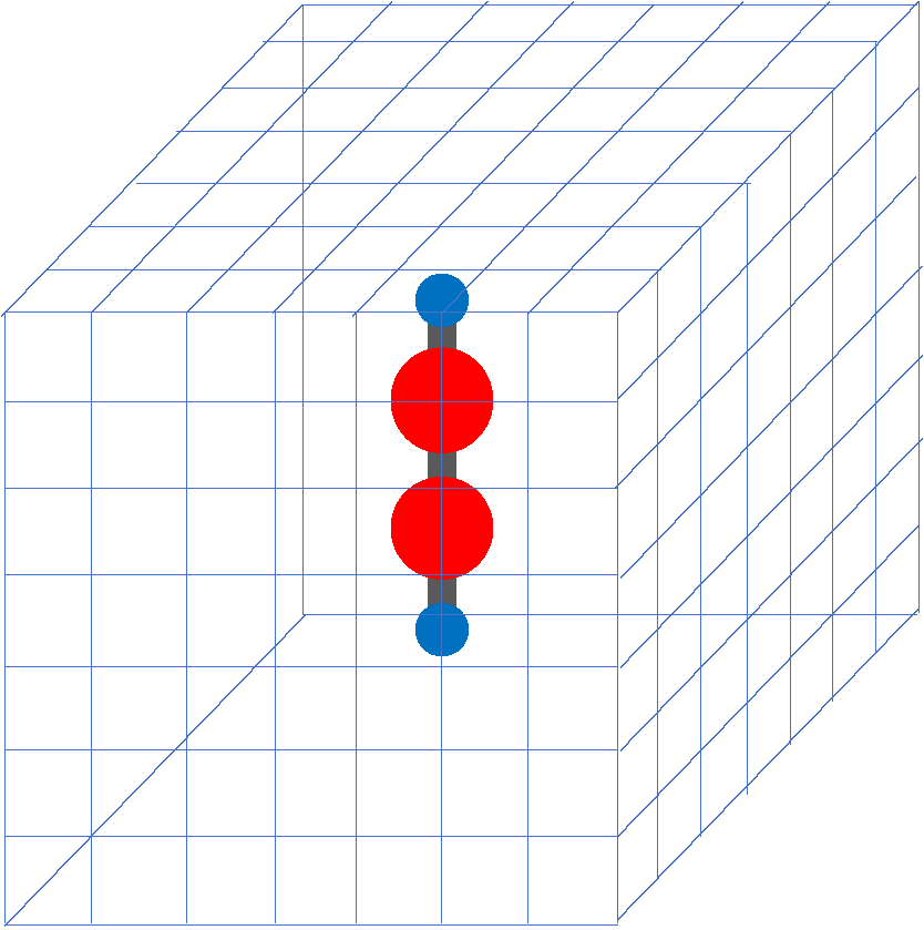
Acetylene molecule is a linear chain molecule composed of two Carbon atoms and two Hydrogen atoms.

In SALMON, we use a three-dimensional (3D) uniform grid system to express physical quantities such as electron orbitals.
Input files
To run the code, following files in the directory SALMON/samples/exercise_01_C2H2_gs/ are used:
| file name | description |
| C2H2_gs.inp | input file that contains input keywords and their values |
| C_rps.dat | pseodupotential file for carbon atom |
| H_rps.dat | pseudopotential file for hydrogen atom |
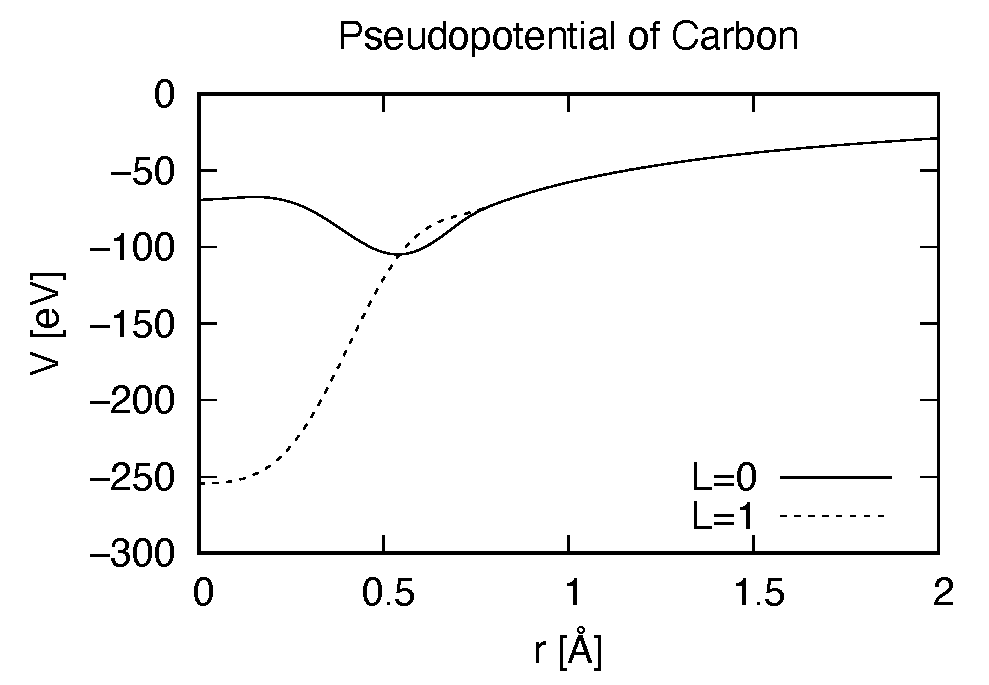
Pseudopotential files are needed for two elements, Carbon (C) and Hydrogen (H). The pseudopoential depends on the angular momentum, and looks as follows (for Carbon).
In the input file C2H2_gs.inp, input keywords are specified.
Most of them are mandatory to execute the ground state calculation.
This will help you to prepare an input file for other systems that you
want to calculate. A complete list of the input keywords that can be
used in the input file can be found in
List of input keywords.
!########################################################################################!
! Excercise 01: Ground state of C2H2 molecule                                            !
!----------------------------------------------------------------------------------------!
! * The detail of this excercise is explained in our manual(see chapter: 'Exercises').   !
!   The manual can be obtained from: https://salmon-tddft.jp/documents.html              !
! * Input format consists of group of keywords like:                                     !
!     &group                                                                             !
!       input keyword = xxx                                                              !
!     /                                                                                  !
!   (see chapter: 'List of input keywords' in the manual)                                !
!----------------------------------------------------------------------------------------!
! * Conversion from unit_system = 'a.u.' to 'A_eV_fs':                                   !
!   Length: 1 [a.u.] = 0.52917721067    [Angstrom]                                       !
!   Energy: 1 [a.u.] = 27.21138505      [eV]                                             !
!   Time  : 1 [a.u.] = 0.02418884326505 [fs]                                             !
!########################################################################################!

&calculation
  !type of theory
  theory = 'dft'
/
&control
  !common name of output files
  sysname = 'C2H2'
/
&units
  !units used in input and output files
  unit_system = 'A_eV_fs'
/
&system
  !periodic boundary condition
  yn_periodic = 'n'

  !number of elements, atoms, electrons and states(orbitals)
  nelem  = 2
  natom  = 4
  nelec  = 10
  nstate = 6
/
&pseudo
  !name of input pseudo potential file
  file_pseudo(1) = './C_rps.dat'
  file_pseudo(2) = './H_rps.dat'

  !atomic number of element
  izatom(1) = 6
  izatom(2) = 1

  !angular momentum of pseudopotential that will be treated as local
  lloc_ps(1) = 1
  lloc_ps(2) = 0
  !--- Caution ---------------------------------------!
  ! Indices must correspond to those in &atomic_coor. !
  !---------------------------------------------------!
/
&functional
  !functional('PZ' is Perdew-Zunger LDA: Phys. Rev. B 23, 5048 (1981).)
  xc = 'PZ'
/
&rgrid
  !spatial grid spacing(x,y,z)
  dl(1:3) = 0.25d0, 0.25d0, 0.25d0

  !number of spatial grids(x,y,z)
  num_rgrid(1:3) = 64, 64, 64
/
&scf
  !maximum number of scf iteration and threshold of convergence
  nscf      = 300
  threshold = 1.0d-9
/
&analysis
  !output of all orbitals, density,
  !density of states, projected density of states,
  !and electron localization function
  yn_out_psi  = 'y'
  yn_out_dns  = 'y'
  yn_out_dos  = 'y'
  yn_out_pdos = 'y'
  yn_out_elf  = 'y'
/
&atomic_coor
  !cartesian atomic coodinates
  'C'    0.000000    0.000000    0.599672  1
  'H'    0.000000    0.000000    1.662257  2
  'C'    0.000000    0.000000   -0.599672  1
  'H'    0.000000    0.000000   -1.662257  2
  !--- Format ---------------------------------------------------!
  ! 'symbol' x y z index(correspond to that of pseudo potential) !
  !--------------------------------------------------------------!
/
Execusion
In a multiprocess environment, calculation will be executed as:
$ mpiexec -n NPROC salmon < C2H2_gs.inp > C2H2_gs.out
where NPROC is the number of MPI processes. A standard output will be stored in the file C2H2_gs.out.
Output files
After the calculation, following output files and a directory are created in the directory that you run the code in addition to the standard output file,
| name | description |
| C2H2_info.data | information on ground state solution |
| C2H2_eigen.data | orbital energies |
| C2H2_k.data | k-point distribution (for isolated systems, only gamma point is described) |
| data_for_restart | directory where files used in the real-time calculation are contained |
| psi_ob1.cube, psi_ob2.cube, ... | electron orbitals |
| dns.cube | a cube file for electron density |
| dos.data | density of states |
| pdos1.data, pdos2.data, ... | projected density of states |
| elf.cube | electron localization function (ELF) |
| PS_C_KY_n.dat | information on pseodupotential file for carbon atom |
| PS_H_KY_n.dat | information on pseodupotential file for hydrogen atom |
We first explain the standard output file. In the beginning of the file, input variables used in the calculation are shown.
##############################################################################
# SALMON: Scalable Ab-initio Light-Matter simulator for Optics and Nanoscience
#
#                             Version 2.0.1
#
##############################################################################
  Libxc: [disabled]
   theory= dft
   use of real value orbitals =  T
 ======
 MPI distribution:
   nproc_k     :           1
   nproc_ob    :           1
   nproc_rgrid :           1           1           2
 OpenMP parallelization:
   number of threads :         256
 .........
After that, the SCF loop starts. At each iteration step, the total energy as well as orbital energies and some other quantities are displayed.
-----------------------------------------------
iter=     1     Total Energy=      -197.59254070     Gap=   -20.17834599     Vh iter= 234
    1       -29.9707      2       -28.3380      3       -13.0123      4         5.8457
    5        -9.9213      6       -14.3326
iter and int_x|rho_i(x)-rho_i-1(x)|dx/nelec        =      1 0.31853198E+00
Ne=   10.0000000000000
-----------------------------------------------
iter=     2     Total Energy=      -280.97950515     Gap=    -9.59770609     Vh iter= 247
    1       -17.4334      2       -24.4941      3       -20.1872      4         0.8020
    5        -3.4058      6        -8.7957
iter and int_x|rho_i(x)-rho_i-1(x)|dx/nelec        =      2 0.54493263E+00
Ne=   10.0000000000000
-----------------------------------------------
iter=     3     Total Energy=      -295.67034640     Gap=    -6.90359156     Vh iter= 229
    1       -16.0251      2       -19.7759      3       -17.6765      4        -0.9015
    5        -2.9323      6        -7.8050
iter and int_x|rho_i(x)-rho_i-1(x)|dx/nelec        =      3 0.13010987E+00
Ne=   10.0000000000000
When the convergence criterion is satisfied, the SCF calculation ends.
-----------------------------------------------
iter=   162     Total Energy=      -339.69525272     Gap=     6.78870999     Vh iter=   1
    1       -18.4106      2       -13.9966      3       -12.4163      4        -7.3386
    5        -7.3386      6        -0.5498
iter and int_x|rho_i(x)-rho_i-1(x)|dx/nelec        =    162 0.50237787E-08
Ne=   9.99999999999999
-----------------------------------------------
iter=   163     Total Energy=      -339.69525269     Gap=     6.78870999     Vh iter=   1
    1       -18.4106      2       -13.9966      3       -12.4163      4        -7.3386
    5        -7.3386      6        -0.5498
iter and int_x|rho_i(x)-rho_i-1(x)|dx/nelec        =    163 0.69880308E-09
Ne=   9.99999999999999
 #GS converged at   164  : 0.69880308E-09
Next, the force acting on ions and some other information related to orbital energies are shown.
===== force =====
    1 -0.33652081E-05  0.16854696E-04 -0.59496450E+00
    2 -0.59222259E-06  0.24915590E-05  0.57651725E+00
    3 -0.37839836E-05  0.20304090E-04  0.59493028E+00
    4 -0.86779607E-06  0.39560274E-05 -0.57651738E+00
orbital energy information-------------------------------
Lowest occupied orbital -0.676576619015730
Highest occupied orbital (HOMO) -0.269686750876529
Lowest unoccupied orbital (LUMO) -2.020624936948345E-002
Highest unoccupied orbital -2.020624936948345E-002
HOMO-LUMO gap  0.249480501507045
Physicaly upper bound of eps(omega)  0.656370369646246
---------------------------------------------------------
Lowest occupied orbital[eV]  -18.4105868958642
Highest occupied orbital (HOMO)[eV]  -7.33855002098465
Lowest unoccupied orbital (LUMO)[eV] -0.549840032009334
Highest unoccupied orbital[eV] -0.549840032009334
HOMO-LUMO gap[eV]   6.78870998897532
Physicaly upper bound of eps(omega)[eV]   17.8607468638548
---------------------------------------------------------
 writing restart data...
 writing completed.
In the directory data_for_restart, files that will be used in the next-step
time evolution calculations are stored.
Other output files include following information.
C2H2_info.data
Calculated orbital and total energies as well as parameters specified in the input file are shown.
C2H2_eigen.data
Orbital energies.
#esp: single-particle energies (eigen energies)
#occ: occupation numbers, io: orbital index
# 1:io, 2:esp[eV], 3:occ
C2H2_k.data
k-point distribution(for isolated systems, only gamma point is described).
# ik: k-point index
# kx,ky,kz: Reduced coordinate of k-points
# wk: Weight of k-point
# 1:ik[none] 2:kx[none] 3:ky[none] 4:kz[none] 5:wk[none]
# coefficients (2*pi/a [a.u.]) in kx, ky, kz
psi_ob1.cube, psi_ob2.cube, ...
Cube files for electron orbitals. The number in the filename indicates the index of the orbital. Atomic unit is adopted in all cube files.
dns.cube
A cube file for electron density.
dos.data
A file for density of states. The units used in this file are affected
by the input parameter, unit_system in &unit.
elf.cube
A cube file for electron localization function (ELF).
We show several image that are created from the output files.
Highest occupied molecular orbital (HOMO)
The output files
psi_ob1.cube,psi_ob2.cube, ... are used to create the image.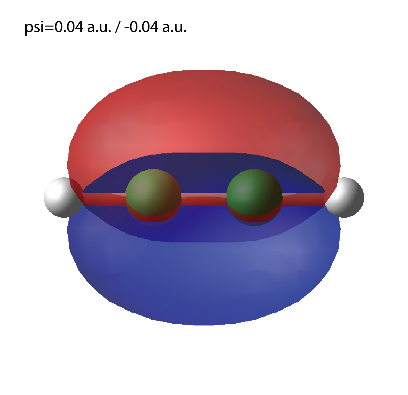
Electron density
The output files
dns.cube, ... are used to create the image.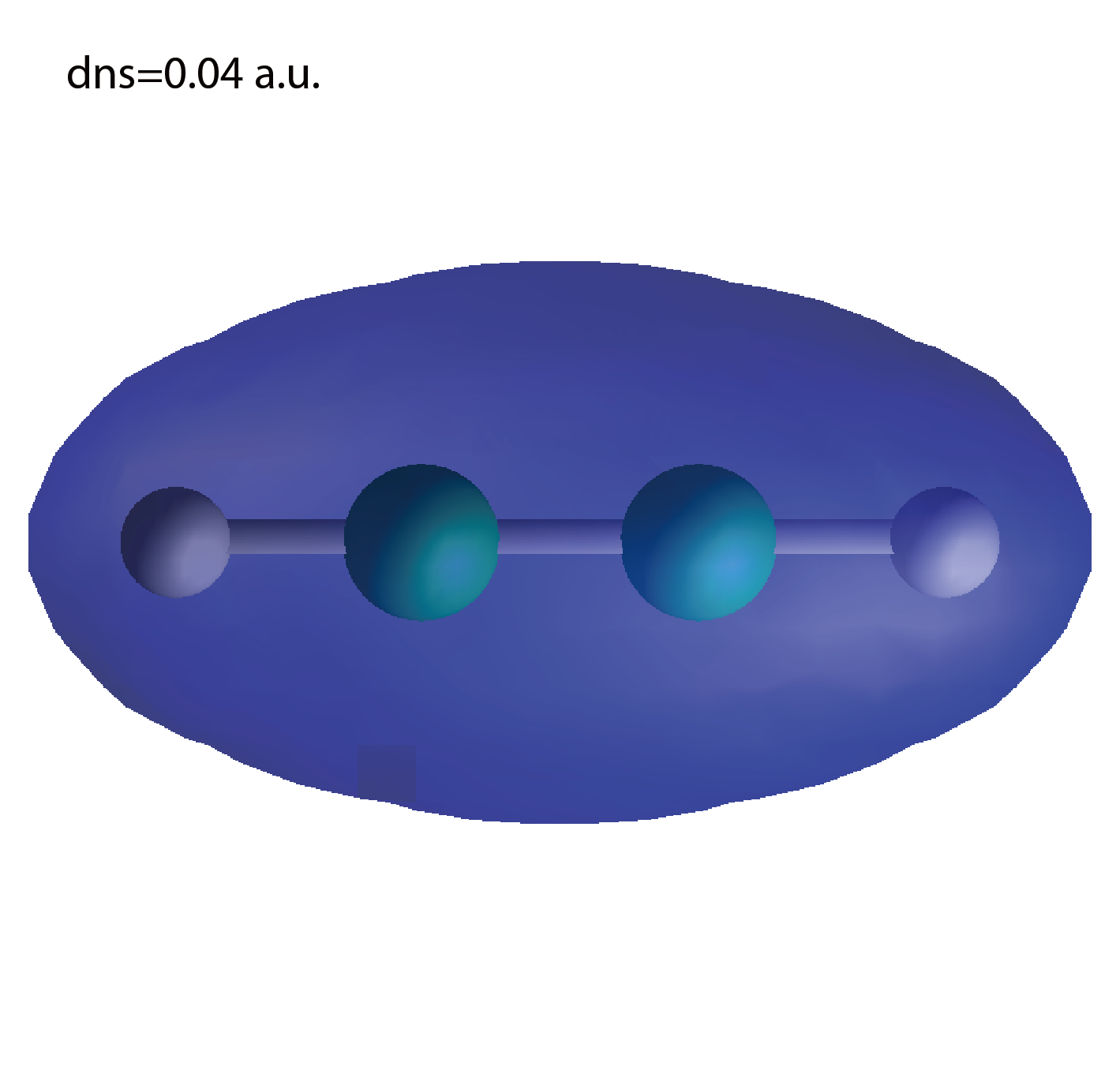
Electron localization function
The output files
elf.cube, ... are used to create the image.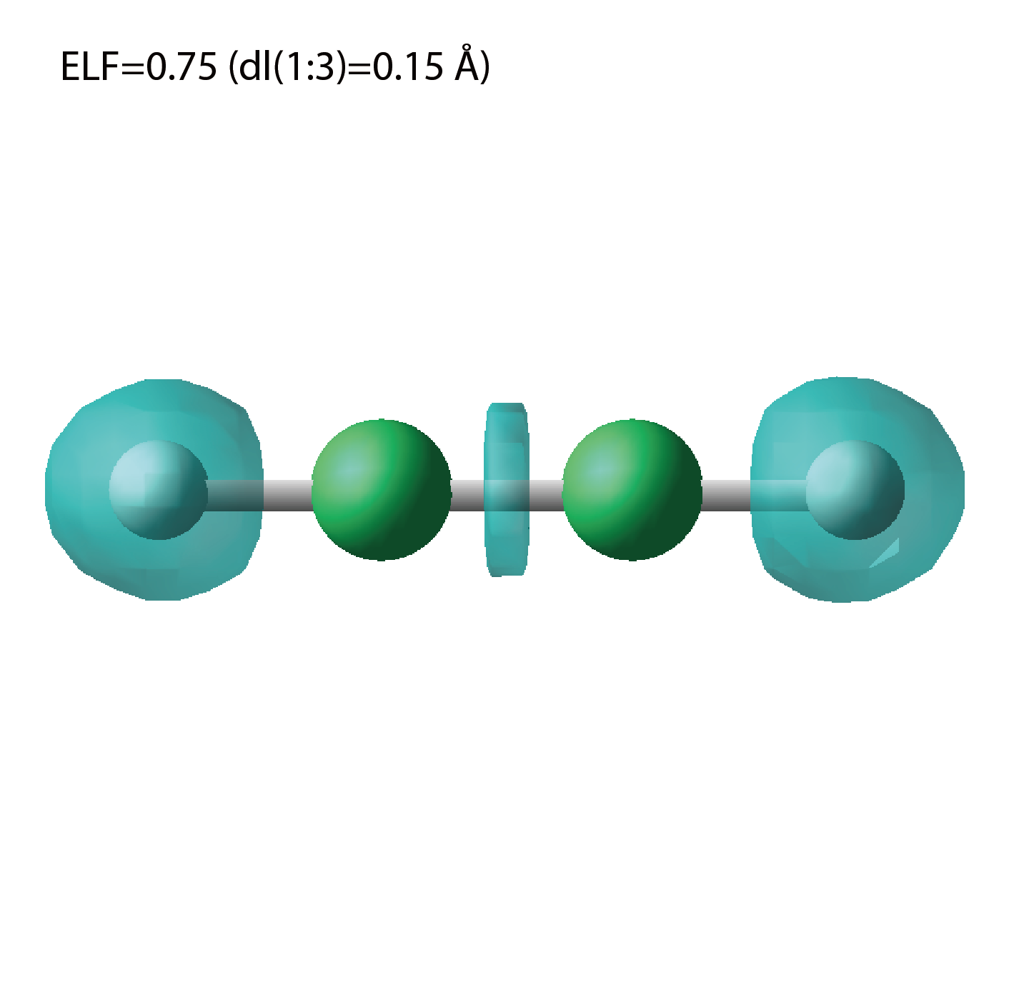
Exercise-2: Polarizability and photoabsorption of C2H2 molecule
In this exercise, we learn the linear response calculation in the acetylene (C2H2) molecule, solving the time-dependent Kohn-Sham equation. The linear response calculation provides the polarizability and the oscillator strength distribution of the molecule. This exercise should be carried out after finishing the ground state calculation that was explained in Exercise-1.
Polarizability \(\alpha_{\mu \nu}(t)\) is the basic quantity that characterizes optical responses of molecules and nano-particles, where \(\mu, \nu\) indicate Cartesian components, \(\mu, \nu = x,y,z\). The polarizability \(\alpha_{\mu \nu}(t)\) relates the \(\mu\) component of the electric dipole moment at time \(t\), \(p_{\mu}(t)\), with the \(\nu\) component of the electric field at time \(t'\),
\(p_{\mu}(t) = \sum_{\nu=x,y,z} \alpha_{\mu \nu}(t-t') E_{\nu}(t').\)
We introduce a frequency-dependent polarizability by the time-frequency Fourier transformation of the polarizability,
\(\tilde \alpha_{\mu \nu}(\omega) = \int dt e^{i\omega t} \alpha_{\mu \nu}(t).\)
The imaginary part of the frequency-dependent polarizability is related to the photoabsorption cross section \(\sigma(\omega)\) by
\(\sigma(\omega) = \frac{4\pi \omega}{c} \frac{1}{3} \sum_{\mu=x,y,z} {\rm Im} \tilde \alpha_{\mu \mu}(\omega).\)
The photoabsorption cross section is also related to the oscillator strength distribution by
\(\sigma(\omega) = \frac{2\pi^2 e^2}{mc} \frac{df(\omega)}{d\omega}.\)
In SALMON, the polarizability is calculated in time domain. First the ground state orbital \(\phi_i(\mathbf{r})\) that satisfies the Kohn-Sham equation,
\(H_{\rm KS} \phi_i(\mathbf{r}) = \epsilon_i \phi_i(\mathbf{r}),\)
is prepared. Then an impulsive force given by the potential
\(V_{\rm ext}(\mathbf{r},t) = I \delta(t) z,\)
is applied to all electrons in the C2H2 molecule along the molecular axis which we take \(z\) axis. \(I\) is the magnitude of the impulse, and \(\delta(t)\) is the Dirac's delta function. The orbital is distorted by the impulsive force at \(t=0\). Immediately after the impulse is applied, the orbital becomes
\(\psi_i(\mathbf{r},t=0_+) = e^{iIz/\hbar} \phi_i(\mathbf{r}).\)
After the impulsive force is applied at \(t=0\), a time evolution calculation is carried out without any external fields,
\(i\hbar \frac{\partial}{\partial t} \psi_i(\mathbf{r},t) = H_{\rm KS}(t) \psi_i(\mathbf{r},t).\)
During the time evolution, the electric dipole moment given by
\(p_z(t) = \int d\mathbf{r} (-ez) \sum_i \vert \psi_i(\mathbf{r},t) \vert^2,\)
is monitored. After the time evolution calculation, a time-frequency Fourier transformation is carried out for the electric dipole moment to obtain the frequency-dependent polarizability by
\(\tilde \alpha_{zz}(\omega) = - \frac{e}{I} \int dt e^{i\omega t} p_z(t).\)
Input files
To run the code, following files are necessary:
| file name | description |
| C2H2_response.inp | input file that contains input keywords and their values |
| C_rps.dat | pseodupotential file for carbon atom |
| H_rps.dat | pseudopotential file for hydrogen atom |
| restart | directory created in the ground
state calculation
(rename the directory from
data_for_restart to restart)
|
First three files are prepared in the directory SALMON/samples/exercise_02_C2H2_lr/.
The file C2H2_rt_response.inp that contains input keywords and their values.
The pseudopotential files should be the same as those used in the ground state calculation.
In the directory restart, those files created in the ground state calculation and stored
in the directory data_for_restart are included.
Therefore, copy the directory as cp -R data_for_restart restart
if you calculate at the same directory as you did the ground state calculation.
In the input file C2H2_rt_response.inp, input keywords are specified.
Most of them are mandatory to execute the linear response calculation.
This will help you to prepare the input file for other systems that you
want to calculate. A complete list of the input keywords that can be
used in the input file can be found in
List of input keywords.
!########################################################################################!
! Excercise 02: Polarizability and photoabsorption of C2H2 molecule                      !
!----------------------------------------------------------------------------------------!
! * The detail of this excercise is explained in our manual(see chapter: 'Exercises').   !
!   The manual can be obtained from: https://salmon-tddft.jp/documents.html              !
! * Input format consists of group of keywords like:                                     !
!     &group                                                                             !
!       input keyword = xxx                                                              !
!     /                                                                                  !
!   (see chapter: 'List of input keywords' in the manual)                                !
!----------------------------------------------------------------------------------------!
! * Conversion from unit_system = 'a.u.' to 'A_eV_fs':                                   !
!   Length: 1 [a.u.] = 0.52917721067    [Angstrom]                                       !
!   Energy: 1 [a.u.] = 27.21138505      [eV]                                             !
!   Time  : 1 [a.u.] = 0.02418884326505 [fs]                                             !
!----------------------------------------------------------------------------------------!
! * Copy the ground state data directory('data_for_restart') (or make symbolic link)     !
!   calculated in 'samples/exercise_01_C2H2_gs/' and rename the directory to 'restart/'  !
!   in the current directory.                                                            !
!########################################################################################!

&calculation
  !type of theory
  theory = 'tddft_response'
/
&control
  !common name of output files
  sysname = 'C2H2'
/
&units
  !units used in input and output files
  unit_system = 'A_eV_fs'
/
&system
  !periodic boundary condition
  yn_periodic = 'n'

  !number of elements, atoms, electrons and states(orbitals)
  nelem  = 2
  natom  = 4
  nelec  = 10
  nstate = 6
/
&pseudo
  !name of input pseudo potential file
  file_pseudo(1) = './C_rps.dat'
  file_pseudo(2) = './H_rps.dat'

  !atomic number of element
  izatom(1) = 6
  izatom(2) = 1

  !angular momentum of pseudopotential that will be treated as local
  lloc_ps(1) = 1
  lloc_ps(2) = 0
  !--- Caution ---------------------------------------!
  ! Indices must correspond to those in &atomic_coor. !
  !---------------------------------------------------!
/
&functional
  !functional('PZ' is Perdew-Zunger LDA: Phys. Rev. B 23, 5048 (1981).)
  xc = 'PZ'
/
&rgrid
  !spatial grid spacing(x,y,z)
  dl(1:3) = 0.25d0, 0.25d0, 0.25d0

  !number of spatial grids(x,y,z)
  num_rgrid(1:3) = 64, 64, 64
/
&tgrid
  !time step size and number of time grids(steps)
  dt = 1.25d-3
  nt = 5000
/
&emfield
  !envelope shape of the incident pulse('impulse': impulsive field)
  ae_shape1 = 'impulse'

  !polarization unit vector(real part) for the incident pulse(x,y,z)
  epdir_re1(1:3) = 0.0d0, 0.0d0, 1.0d0
  !--- Caution ---------------------------------------------------------!
  ! Definition of the incident pulse is written in:                     !
  ! https://www.sciencedirect.com/science/article/pii/S0010465518303412 !
  !---------------------------------------------------------------------!
/
as_shape1='impulse' is used. It indicates that a weak impulsive perturbation is applied at \(t=0\).&analysis
!energy grid size and number of energy grids for output files
de = 1.0d-2
nenergy = 3000
/
&atomic_coor
  !cartesian atomic coodinates
  'C'    0.000000    0.000000    0.599672  1
  'H'    0.000000    0.000000    1.662257  2
  'C'    0.000000    0.000000   -0.599672  1
  'H'    0.000000    0.000000   -1.662257  2
  !--- Format ---------------------------------------------------!
  ! 'symbol' x y z index(correspond to that of pseudo potential) !
  !--------------------------------------------------------------!
/
Execusion
Before execusion, remember to copy the directory restart that is created in the ground
state calculation as data_for_restart in the present directory.
In a multiprocess environment, calculation will be executed as:
$ mpiexec -n NPROC salmon < C2H2_rt_response.inp > C2H2_rt_response.out
where NPROC is the number of MPI processes.
A standard output will be stored in the file C2H2_rt_response.out.
Output files
After the calculation, following output files are created in the directory that you run the code in addition to the standard output file,
| file name | description |
| C2H2_response.data | polarizability and oscillator strength distribution as functions of energy |
| C2H2_rt.data | components of
change of dipole moment
(electrons/plus definition)
and total dipole moment
(electrons/minus + ions/plus)
as functions of time
|
| C2H2_rt_energy.data | total energy and electronic excitation energy as functions of time |
| PS_C_KY_n.dat | information on pseodupotential file for carbon atom |
| PS_H_KY_n.dat | information on pseodupotential file for hydrogen atom |
We first explain the standard output file. In the beginning of the file, input variables used in the calculation are shown.
##############################################################################
# SALMON: Scalable Ab-initio Light-Matter simulator for Optics and Nanoscience
#
#                             Version 2.0.1
##############################################################################
  Libxc: [disabled]
   theory= tddft_response

 Total time step      =        5000
 Time step[fs]        =  1.250000000000000E-003
 Energy range         =        3000
 Energy resolution[eV]=  1.000000000000000E-002
 Field strength[a.u.] =  1.000000000000000E-002
   use of real value orbitals =  F
 ======
 .........
After that, the time evolution loop starts. At every 10 iteration steps, the time, dipole moments in three Cartesian directions, the total number of electrons, the total energy, and the number of iterations solving the Poisson equation are displayed.
 time-step    time[fs]                           Dipole moment(xyz)[A]      electrons  Total energy[eV]    iterVh
#----------------------------------------------------------------------
      10    0.01250000 -0.56521137E-07 -0.28812833E-07 -0.25558983E-01    10.00000000     -339.68150366   34
      20    0.02500000 -0.19835467E-06 -0.10147641E-06 -0.45169126E-01     9.99999999     -339.68147442   49
      30    0.03750000 -0.37937911E-06 -0.19537418E-06 -0.57843871E-01     9.99999999     -339.68146891   45
      40    0.05000000 -0.56465010E-06 -0.29324906E-06 -0.64072126E-01     9.99999999     -339.68146804   38
      50    0.06250000 -0.73343753E-06 -0.38431758E-06 -0.65208422E-01     9.99999999     -339.68146679   25
      60    0.07500000 -0.87559727E-06 -0.46276791E-06 -0.62464066E-01     9.99999999     -339.68146321   35
      70    0.08750000 -0.98769124E-06 -0.52594670E-06 -0.56740338E-01     9.99999998     -339.68145535   20
      80    0.10000000 -0.10701350E-05 -0.57309375E-06 -0.48483747E-01     9.99999998     -339.68144840   40
      90    0.11250000 -0.11253992E-05 -0.60455485E-06 -0.38296037E-01     9.99999998     -339.68144186   21
Explanations of other output files are given below:
C2H2_rt.data
Results of time evolution calculation for vector potential, electric field, and dipole moment. In the first several lines, explanations of included data are given.
# Real time calculation:
# Ac_ext: External vector potential field
# E_ext: External electric field
# Ac_tot: Total vector potential field
# E_tot: Total electric field
# ddm_e: Change of dipole moment (electrons/plus definition)
# dm: Total dipole moment (electrons/minus + ions/plus)
# 1:Time[fs] 2:Ac_ext_x[fs*V/Angstrom] 3:Ac_ext_y[fs*V/Angstrom] 4:Ac_ext_z[fs*V/Angstrom]
# 5:E_ext_x[V/Angstrom] 6:E_ext_y[V/Angstrom] 7:E_ext_z[V/Angstrom]
# 8:Ac_tot_x[fs*V/Angstrom] 9:Ac_tot_y[fs*V/Angstrom] 10:Ac_tot_z[fs*V/Angstrom]
# 11:E_tot_x[V/Angstrom] 12:E_tot_y[V/Angstrom] 13:E_tot_z[V/Angstrom]
# 14:ddm_e_x[Angstrom] 15:ddm_e_y[Angstrom] 16:ddm_e_z[Angstrom] 17:dm_x[Angstrom]
# 18:dm_y[Angstrom] 19:dm_z[Angstrom]
Using first column (time in femtosecond) and 19th column (dipole moment in \(z\) direction), the following graph can be drawn.
The dipole moment shows oscillations in femtosecond time scale that reflec electronic excitations.
C2H2_response.data
Time-frequency Fourier transformation of the dipole moment gives the polarizability and the strength function.
# Fourier-transform spectra:
# alpha: Polarizability
# df/dE: Strength function
# 1:Energy[eV] 2:Re(alpha_x)[Augstrom^2/V] 3:Re(alpha_y)[Augstrom^2/V]
# 4:Re(alpha_z)[Augstrom^2/V] 5:Im(alpha_x)[Augstrom^2/V] 6:Im(alpha_y)[Augstrom^2/V]
# 7:Im(alpha_z)[Augstrom^2/V] 8:df_x/dE[none] 9:df_y/dE[none] 10:df_z/dE[none]
Using first column (energy in electron-volt) and 10th column (oscillator strength distribution in \(z\) direction), the following graph can be drawn.
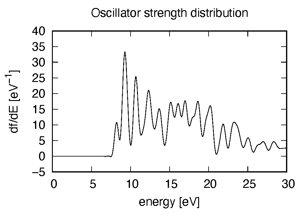
There appears many peaks above the HOMO-LUMO gap energy. The strong excitation appears at around 9.3 eV.
C2H2_rt_energy.data
Energies are stored as functions of time.
# Real time calculation:
# Eall: Total energy
# Eall0: Initial energy
# 1:Time[fs] 2:Eall[eV] 3:Eall-Eall0[eV]
Eall and Eall-Eall0 are total energy and electronic excitation energy, respectively.
Exercise-3: Electron dynamics in C2H2 molecule under a pulsed electric field
In this exercise, we learn the calculation of the electron dynamics in the acetylene (C2H2) molecule under a pulsed electric field, solving the time-dependent Kohn-Sham equation. As outputs of the calculation, such quantities as the total energy and the electric dipole moment of the system as functions of time are calculated. This tutorial should be carried out after finishing the ground state calculation that was explained in Exercise-1.
In the calculation, a pulsed electric field specified by the following vector potential will be used,
\(A(t) = - \frac{E_0}{\omega} \hat z \cos^2 \frac{\pi}{T} \left( t - \frac{T}{2} \right) \sin \omega \left( t - \frac{T}{2} \right), \hspace{5mm} (0 < t < T).\)
The electric field is given by \(E(t) = -(1/c)(dA(t)/dt)\). The parameters that characterize the pulsed field such as the amplitude \(E_0\), frequency \(\omega\), pulse duration \(T\), polarization direction \(\hat z\), are specified in the input file. In the time dependent Kohn-Sham equation, the external field is included as the scalar potential, \(V_{\rm ext}(\mathbf{r},t) = eE(t)z\).
Input files
To run the code, following files are necessary:
| file name | description |
| C2H2_rt_pulse.inp | input file that contain input keywords and their values. |
| C_rps.dat | pseodupotential file for carbon |
| H_rps.dat | pseudopotential file for hydrogen |
| restart | directory created in the ground state calculation
(rename the directory from data_for_restart to restart)
|
First three files are prepared in the directory SALMON/samples/exercise_03_C2H2_rt/.
The file C2H2_rt_pulse.inp that contains input keywords and their values.
The pseudopotential files should be the same as those used in the ground state calculation.
In the directory restart, those files created in the ground state calculation and stored
in the directory data_for_restart are included.
Therefore, copy the directory as cp -R data_for_restart restart
if you calculate at the same directory as you did the ground state calculation.
In the input file C2H2_rt_pulse.inp, input keywords are specified.
Most of them are mandatory to execute the calculation of
electron dynamics induced by a pulsed electric field.
This will help you to prepare the input file for other systems and other
pulsed electric fields that you want to calculate. A complete list of
the input keywords that can be used in the input file can be found in
List of input keywords.
!########################################################################################!
! Excercise 03:  Electron dynamics in C2H2 molecule under a pulsed electric field        !
!----------------------------------------------------------------------------------------!
! * The detail of this excercise is explained in our manual(see chapter: 'Exercises').   !
!   The manual can be obtained from: https://salmon-tddft.jp/documents.html              !
! * Input format consists of group of keywords like:                                     !
!     &group                                                                             !
!       input keyword = xxx                                                              !
!     /                                                                                  !
!   (see chapter: 'List of input keywords' in the manual)                                !
!----------------------------------------------------------------------------------------!
! * Conversion from unit_system = 'a.u.' to 'A_eV_fs':                                   !
!   Length: 1 [a.u.] = 0.52917721067    [Angstrom]                                       !
!   Energy: 1 [a.u.] = 27.21138505      [eV]                                             !
!   Time  : 1 [a.u.] = 0.02418884326505 [fs]                                             !
!----------------------------------------------------------------------------------------!
! * Copy the ground state data directory('data_for_restart') (or make symbolic link)     !
!   calculated in 'samples/exercise_01_C2H2_gs/' and rename the directory to 'restart/'  !
!   in the current directory.                                                            !
!########################################################################################!

&calculation
  !type of theory
  theory = 'tddft_pulse'
/
&control
  !common name of output files
  sysname = 'C2H2'
/
&units
  !units used in input and output files
  unit_system = 'A_eV_fs'
/
&system
  !periodic boundary condition
  yn_periodic = 'n'

  !number of elements, atoms, electrons and states(orbitals)
  nelem  = 2
  natom  = 4
  nelec  = 10
  nstate = 6
/
&pseudo
  !name of input pseudo potential file
  file_pseudo(1) = './C_rps.dat'
  file_pseudo(2) = './H_rps.dat'

  !atomic number of element
  izatom(1) = 6
  izatom(2) = 1

  !angular momentum of pseudopotential that will be treated as local
  lloc_ps(1) = 1
  lloc_ps(2) = 0
  !--- Caution ---------------------------------------!
  ! Indices must correspond to those in &atomic_coor. !
  !---------------------------------------------------!
/
&functional
  !functional('PZ' is Perdew-Zunger LDA: Phys. Rev. B 23, 5048 (1981).)
  xc = 'PZ'
/
&rgrid
  !spatial grid spacing(x,y,z)
  dl(1:3) = 0.25d0, 0.25d0, 0.25d0

  !number of spatial grids(x,y,z)
  num_rgrid(1:3) = 64, 64, 64
/
&tgrid
  !time step size and number of time grids(steps)
  dt = 1.25d-3
  nt = 5000
/
&emfield
  !envelope shape of the incident pulse('Ecos2': cos^2 type envelope for scalar potential)
  ae_shape1 = 'Acos2'

  !peak intensity(W/cm^2) of the incident pulse
  I_wcm2_1 = 5.00d13

  !duration of the incident pulse
  tw1 = 6.00d0

  !mean photon energy(average frequency multiplied by the Planck constant) of the incident pulse
  omega1 = 3.10d0

  !polarization unit vector(real part) for the incident pulse(x,y,z)
  epdir_re1(1:3) = 0.00d0, 0.00d0, 1.00d0
  !--- Caution ---------------------------------------------------------!
  ! Definition of the incident pulse is written in:                     !
  ! https://www.sciencedirect.com/science/article/pii/S0010465518303412 !
  !---------------------------------------------------------------------!
/
&analysis
  !energy grid size and number of energy grids for output files
  de      = 1.0d-2
  nenergy = 10000
/
&atomic_coor
  !cartesian atomic coodinates
  'C'    0.000000    0.000000    0.599672  1
  'H'    0.000000    0.000000    1.662257  2
  'C'    0.000000    0.000000   -0.599672  1
  'H'    0.000000    0.000000   -1.662257  2
  !--- Format ---------------------------------------------------!
  ! 'symbol' x y z index(correspond to that of pseudo potential) !
  !--------------------------------------------------------------!
/
Execusion
Before execusion, remember to copy the directory restart that is created in the ground
state calculation as data_for_restart in the present directory.
In a multiprocess environment, calculation will be executed as:
$ mpiexec -n NPROC salmon < C2H2_rt_pulse.inp > C2H2_rt_pulse.out
where NPROC is the number of MPI processes.
A standard output will be stored in the file C2H2_rt_pulse.out.
Output files
After the calculation, following output files are created in the directory that you run the code in addition to the standard output file,
| file name | description |
| C2H2_pulse.data | time-frequency Fourier transform of dipole moment |
| C2H2_rt.data | components of
change of dipole moment
(electrons/plus definition)
and total dipole moment
(electrons/minus + ions/plus)
as functions of time
|
| C2H2_rt_energy.data | total energy and electronic excitation energy as functions of time |
| PS_C_KY_n.dat | information on pseodupotential file for carbon atom |
| PS_H_KY_n.dat | information on pseodupotential file for hydrogen atom |
We first explain the standard output file. In the beginning of the file, input variables used in the calculation are shown.
##############################################################################
# SALMON: Scalable Ab-initio Light-Matter simulator for Optics and Nanoscience
#
#                             Version 2.0.1
##############################################################################
  Libxc: [disabled]
   theory= tddft_pulse

 Total time step      =        5000
 Time step[fs]        =  1.250000000000000E-003
 Energy range         =       10000
 Energy resolution[eV]=  1.000000000000000E-002
Laser frequency     = 3.10[eV]
Pulse width of laser=      6.00000000[fs]
Laser intensity     =  0.50000000E+14[W/cm^2]
   use of real value orbitals =  F
 ======
 ........
After that, the time evolution loop starts. At every 10 iteration steps, the time, dipole moments in three Cartesian directions, the total number of electrons, the total energy, and the number of iterations solving the Poisson equation are displayed.
 time-step    time[fs]                           Dipole moment(xyz)[A]      electrons  Total energy[eV]    iterVh
#----------------------------------------------------------------------
      10    0.01250000 -0.57275542E-07 -0.29197105E-07 -0.74600728E-06    10.00000000     -339.69524047    1
      20    0.02500000 -0.20616352E-06 -0.10537273E-06 -0.10256205E-04    10.00000000     -339.69524348    1
      30    0.03750000 -0.40063325E-06 -0.20597522E-06 -0.47397133E-04    10.00000000     -339.69524090    3
      40    0.05000000 -0.59093535E-06 -0.30630513E-06 -0.13774845E-03    10.00000000     -339.69524287    1
      50    0.06250000 -0.75588343E-06 -0.39552925E-06 -0.31097825E-03    10.00000000     -339.69523949    5
      60    0.07500000 -0.89221538E-06 -0.47142217E-06 -0.59735355E-03    10.00000000     -339.69523784   11
      70    0.08750000 -0.99769538E-06 -0.53192187E-06 -0.10253308E-02    10.00000000     -339.69523285    5
      80    0.10000000 -0.10738281E-05 -0.57676878E-06 -0.16195168E-02     9.99999999     -339.69522482   19
      90    0.11250000 -0.11250289E-05 -0.60722757E-06 -0.23985719E-02     9.99999999     -339.69521092    2
Explanations of other output files are given below:
C2H2_rt.data
Results of time evolution calculation for vector potential, electric field, and dipole moment. In the first several lines, explanations of data included data are given.
# Real time calculation:
# Ac_ext: External vector potential field
# E_ext: External electric field
# Ac_tot: Total vector potential field
# E_tot: Total electric field
# ddm_e: Change of dipole moment (electrons/plus definition)
# dm: Total dipole moment (electrons/minus + ions/plus)
# 1:Time[fs] 2:Ac_ext_x[fs*V/Angstrom] 3:Ac_ext_y[fs*V/Angstrom] 4:Ac_ext_z[fs*V/Angstrom]
# 5:E_ext_x[V/Angstrom] 6:E_ext_y[V/Angstrom] 7:E_ext_z[V/Angstrom]
# 8:Ac_tot_x[fs*V/Angstrom] 9:Ac_tot_y[fs*V/Angstrom] 10:Ac_tot_z[fs*V/Angstrom]
# 11:E_tot_x[V/Angstrom] 12:E_tot_y[V/Angstrom] 13:E_tot_z[V/Angstrom]
# 14:ddm_e_x[Angstrom] 15:ddm_e_y[Angstrom] 16:ddm_e_z[Angstrom] 17:dm_x[Angstrom]
# 18:dm_y[Angstrom] 19:dm_z[Angstrom]
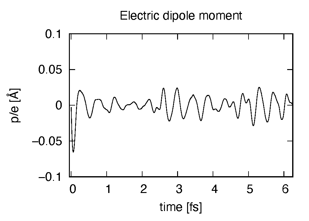
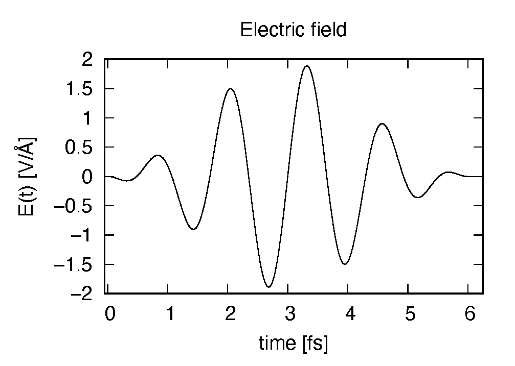
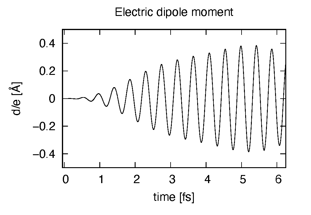
The applied electric field is drawn using the first column (time in femtosecond) and the 7th column (electric field in \(z\) direction in Volt per Angstrom).
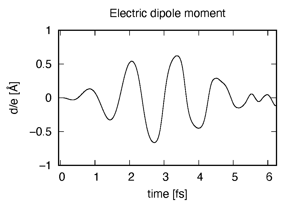
The induced dipole moment is drawn using the first column (time in femtosecond) and 19th column (dipole moment in \(z\) direction). It shows an oscillation similar to the applied electric field. However, the response is not linear since the applied electric field is rather strong.
C2H2_pulse.data
Time-frequency Fourier transformation of the dipole moment. In the first several lines, explanations of data included data are given.
# Fourier-transform spectra:
# energy: Frequency
# dm: Dopile moment
# 1:energy[eV] 2:Re(dm_x)[fs*Angstrom] 3:Re(dm_y)[fs*Angstrom] 4:Re(dm_z)[fs*Angstrom]
# 5:Im(dm_x)[fs*Angstrom] 6:Im(dm_y)[fs*Angstrom] 7:Im(dm_z)[fs*Angstrom]
# 8:|dm_x|^2[fs^2*Angstrom^2] 9:|dm_y|^2[fs^2*Angstrom^2] 10:|dm_z|^2[fs^2*Angstrom^2]
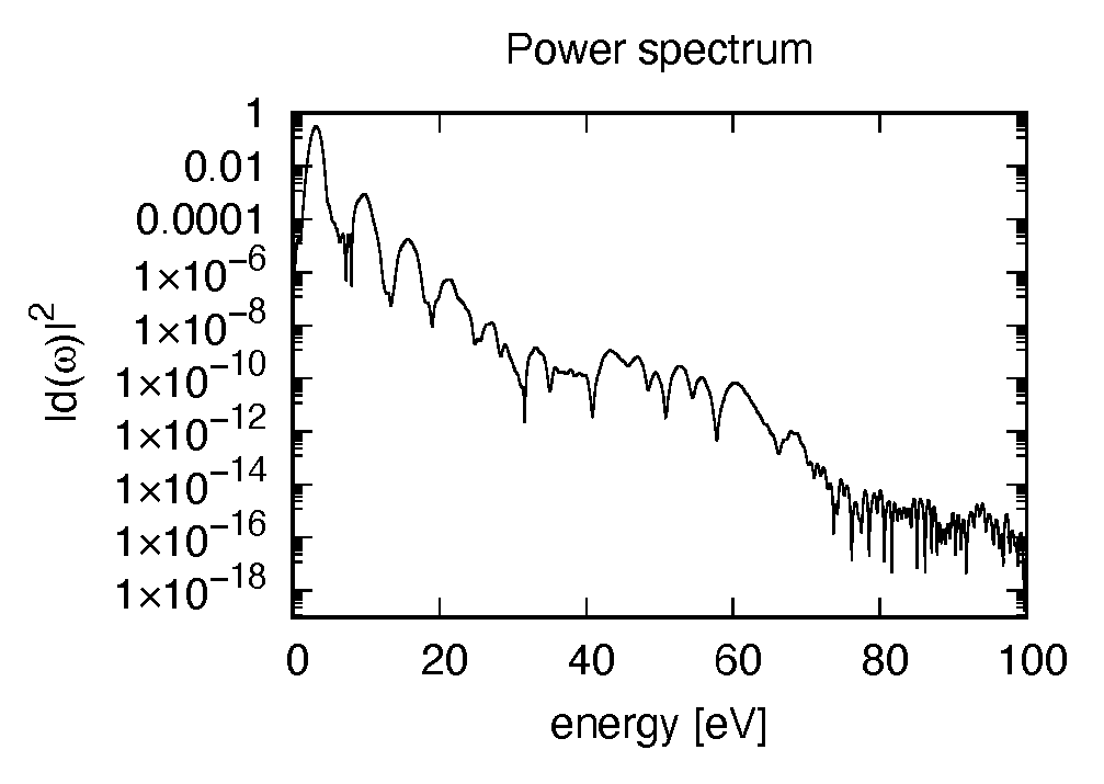
The spectrum of the induced dipole moment, \(|d(\omega)|^2\) is shown in logarithmic scale as a function of the energy, \(\hbar \omega\). High harmonic generations are visible in the spectrum.
C2H2_rt_energy.data
Energies are stored as functions of time. In the first several lines, explanations of data included data are given.
# Real time calculation:
# Eall: Total energy
# Eall0: Initial energy
# 1:Time[fs] 2:Eall[eV] 3:Eall-Eall0[eV]
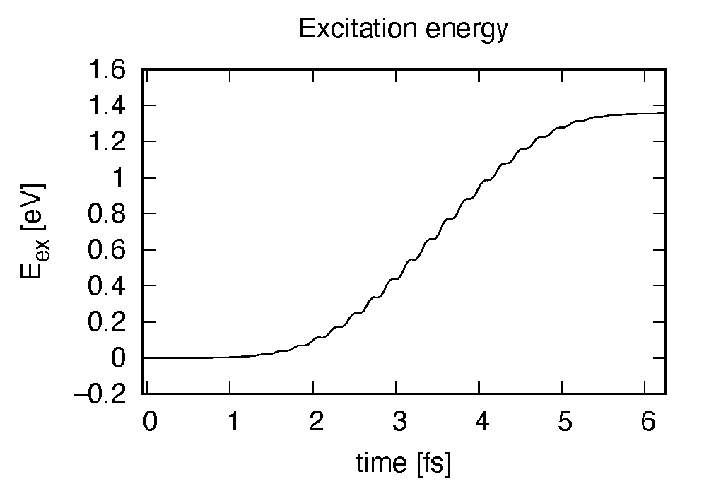
Eall and Eall-Eall0 are total energy and electronic excitation energy, respectively. The figure below shows the electronic excitation energy as a function of time, using the first column (time in femtosecond) and the 3rd column (Eall-Eall0). Although the frequency is below the HOMO-LUMO gap energy, electronic excitations take place because of nonlinear absorption process.
Additional exercise
If we change parameters of the applied electric field, we find a drastic change
in the electronic excitations. In the example below, we increase the intensity
from I_wcm2_1 = 5.00d13 to I_wcm2_1 = 1.00d12 and changes the frequency
from omega1 = 3.10d0 to omega1 = 9.28d0. The new frequency corresponds
to the resonant excitation energy seen in the linear response analysis shown in
in Exercise-2.
The change in the input file is shown below.
&emfield
  !envelope shape of the incident pulse('Ecos2': cos^2 type envelope for scalar potential)
  ae_shape1 = 'Acos2'

  !peak intensity(W/cm^2) of the incident pulse
  I_wcm2_1 = 1.00d12

  !duration of the incident pulse
  tw1 = 6.00d0

  !mean photon energy(average frequency multiplied by the Planck constant) of the incident pulse
  omega1 = 9.28d0

  !polarization unit vector(real part) for the incident pulse(x,y,z)
  epdir_re1(1:3) = 0.00d0, 0.00d0, 1.00d0
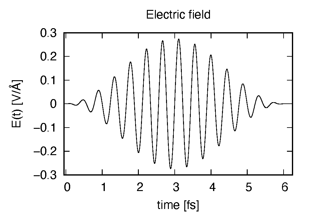
The applied electric field shows a rapid oscillation.
The induced dipole moment also shows a rapid oscillation and does not decrease even though the electric field decreases. This is because the frequency of the applied electric field coincides with the excitation energy of the molecule.
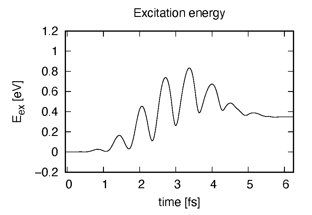
The electronic excitation energy also shows a monotonic increase. Although the strength of the applied electric field is much smaller than the previous case, the amount of the excitation energy is larger, again due to the resonant excitation.
Crystalline silicon (periodic solids)
Exercise-4: Ground state of crystalline silicon
In this exercise, we learn the the ground state calculation of the crystalline silicon that has a diamond structure. A cubic unit cell that contains eight silicon atoms is adopted in the calculation.
This exercise will be useful to learn how to set up calculations in SALMON for any periodic systems such as crystalline solid.
Input files
To run the code, following files in the directory SALMON/samples/exercise_04_bulkSi_gs/ are used:
| file name | description |
| Si_gs.inp | input file that contains input keywords and their values |
| Si_rps.dat | pseodupotential file for silicon atom |
In the input file Si_gs.inp, input keywords are specified.
Most of them are mandatory to execute the ground state calculation.
This will help you to prepare an input file for other systems that you
want to calculate. A complete list of the input keywords that can be
used in the input file can be found in
List of input keywords.
!########################################################################################!
! Excercise 04: Ground state of crystalline silicon(periodic solids)                     !
!----------------------------------------------------------------------------------------!
! * The detail of this excercise is explained in our manual(see chapter: 'Exercises').   !
!   The manual can be obtained from: https://salmon-tddft.jp/documents.html              !
! * Input format consists of group of keywords like:                                     !
!     &group                                                                             !
!       input keyword = xxx                                                              !
!     /                                                                                  !
!   (see chapter: 'List of input keywords' in the manual)                                !
!----------------------------------------------------------------------------------------!
! * Conversion from unit_system = 'a.u.' to 'A_eV_fs':                                   !
!   Length: 1 [a.u.] = 0.52917721067    [Angstrom]                                       !
!   Energy: 1 [a.u.] = 27.21138505      [eV]                                             !
!   Time  : 1 [a.u.] = 0.02418884326505 [fs]                                             !
!########################################################################################!

&calculation
  !type of theory
  theory = 'dft'
/
&control
  !common name of output files
  sysname = 'Si'
/
&units
  !units used in input and output files
  unit_system = 'A_eV_fs'
/
&system
  !periodic boundary condition
  yn_periodic = 'y'

  !grid box size(x,y,z)
  al(1:3) = 5.43d0, 5.43d0, 5.43d0

  !number of elements, atoms, electrons and states(bands)
  nelem  = 1
  natom  = 8
  nelec  = 32
  nstate = 32
/
&pseudo
  !name of input pseudo potential file
  file_pseudo(1) = './Si_rps.dat'

  !atomic number of element
  izatom(1) = 14

  !angular momentum of pseudopotential that will be treated as local
  lloc_ps(1) = 2
  !--- Caution -------------------------------------------!
  ! Index must correspond to those in &atomic_red_coor.   !
  !-------------------------------------------------------!
/
&functional
  !functional('PZ' is Perdew-Zunger LDA: Phys. Rev. B 23, 5048 (1981).)
  xc = 'PZ'
/
&rgrid
  !number of spatial grids(x,y,z)
  num_rgrid(1:3) = 12, 12, 12
/
&kgrid
  !number of k-points(x,y,z)
  num_kgrid(1:3) = 4, 4, 4
/
&scf
  !maximum number of scf iteration and threshold of convergence
  nscf      = 300
  threshold = 1.0d-9
/
&atomic_red_coor
  !cartesian atomic reduced coodinates
  'Si'       .0      .0      .0      1
  'Si'       .25     .25     .25     1
  'Si'       .5      .0      .5      1
  'Si'       .0      .5      .5      1
  'Si'       .5      .5      .0      1
  'Si'       .75     .25     .75     1
  'Si'       .25     .75     .75     1
  'Si'       .75     .75     .25     1
  !--- Format ---------------------------------------------------!
  ! 'symbol' x y z index(correspond to that of pseudo potential) !
  !--------------------------------------------------------------!
/
Execusion
In a multiprocess environment, calculation will be executed as:
$ mpiexec -n NPROC salmon < Si_gs.inp > Si_gs.out
where NPROC is the number of MPI processes. A standard output will be stored in the file Si_gs.out.
Output files
After the calculation, following output files and a directory are created in the directory that you run the code in addition to the standard output file,
| name | description |
| Si_info.data | information on ground state solution |
| Si_eigen.data | energy eigenvalues of orbitals |
| Si_k.data | k-point distribution |
| PS_Si_KY_n.dat | information on pseodupotential file for silicon atom |
| data_for_restart | directory where files used in the real-time calculation are contained |
data_for_restart) from:We first explain the standard output file. In the beginning of the file, input variables used in the calculation are shown.
##############################################################################
# SALMON: Scalable Ab-initio Light-Matter simulator for Optics and Nanoscience
#
#                             Version 2.0.1
##############################################################################
  Libxc: [disabled]
   theory= dft
   use of real value orbitals =  F
 r-space parallelization: off
 ======
 MPI distribution:
   nproc_k     :          16
   nproc_ob    :           1
   nproc_rgrid :           1           1           1
 OpenMP parallelization:
   number of threads :          64
 .........
After that, the SCF loop starts. At each iteration step, the total energy as well as orbital energies and some other quantities are displayed.
-----------------------------------------------
 iter=     1     Total Energy=       314.78493406     Gap=   -95.88543131
 k=           1
     1        37.5762      2        63.8589      3        58.1850      4        43.0042
     5        61.5347      6        29.5604      7        41.5986      8        39.3545
     9        48.5641     10        68.0003     11        75.5196     12        85.4113
 ..........
    21        94.1224     22        53.0821     23        72.0170     24        46.7797
    25        88.6077     26        98.2698     27        42.8071     28        65.0812
    29        60.3648     30        39.6787     31        83.5629     32        62.7365

 iter and int_x|rho_i(x)-rho_i-1(x)|dx/nelec        =      1 0.49478519E+00
 Ne=   32.0000000000000
 -----------------------------------------------
 iter=     2     Total Energy=        62.72724688     Gap=   -77.31200657
 k=           1
     1        14.4913      2        32.6869      3        30.3561      4        20.6816
     5        30.3907      6        16.9184      7        22.2967      8        18.5338
     9        29.0117     10        41.9687     11        42.3490     12        54.6262
..........
When the convergence criterion is satisfied, the SCF calculation ends.
 iter=    60     Total Energy=      -850.76385275     Gap=     1.06020364
 k=           1
     1        -3.7745      2        -3.0158      3        -3.0158      4        -3.0158
     5        -0.4300      6        -0.4300      7        -0.4300      8         0.3765
     9         3.9530     10         3.9530     11         3.9530     12         4.6110
..........
    21         9.6233     22         9.6233     23         9.6956     24         9.9111
    25        11.0259     26        11.0259     27        11.4165     28        11.5976
    29        11.9826     30        11.9887     31        12.0967     32        12.3585

 iter and int_x|rho_i(x)-rho_i-1(x)|dx/nelec        =     60 0.77889300E-09
 Ne=   32.0000000000000
  #GS converged at    61  : 0.77889300E-09
 ===== force =====
     1  0.60775985E-08  0.15425240E-07 -0.22474791E-07
     2 -0.10689345E-06  0.88233132E-07  0.35122981E-09
     3  0.39762202E-07 -0.23921918E-07  0.11855231E-07
     4 -0.79441825E-07 -0.28978042E-07 -0.34109698E-07
     5  0.37990526E-07  0.67211638E-08  0.20384753E-07
     6  0.96418986E-07 -0.70404285E-07  0.10198912E-06
     7  0.16145540E-07  0.30561301E-07 -0.63738382E-07
     8  0.26042178E-07  0.30977639E-07 -0.40587816E-07
 band information-----------------------------------------
 Bottom of VB -0.194818046940532
 Top of VB  0.216611832367042
 Bottom of CB  0.255573599266334
 Top of CB  0.533770712688357
 Fundamental gap  3.896176689929157E-002
 BG between same k-point  3.896176691206812E-002
 Physicaly upper bound of CB for DOS  0.453918744010958
 Physicaly upper bound of eps(omega)  0.609598295602846
 ---------------------------------------------------------
 Bottom of VB[eV]  -5.30126888998779
 Top of VB[eV]   5.89430797692564
 Bottom of CB[eV]   6.95451161825061
 Top of CB[eV]   14.5246403913758
 Fundamental gap[eV]   1.06020364132497
 BG between same k-point[eV]   1.06020364167264
 Physicaly upper bound of CB for DOS[eV]   12.3517577246945
 Physicaly upper bound of eps(omega)[eV]   16.5880139474728
 ---------------------------------------------------------
  writing restart data...
  writing completed.
In the directory data_for_restart, files that will be used in the next-step
time evolution calculations are stored.
Other output files include following information.
Si_info.data
Orbital and total energies as well as parameters specified in the input file.
Total number of iteration =           60

Number of states =           32
Number of electrons =           32

Total energy (eV) =   -850.763852754463
1-particle energies (eV)
    1        -3.7745      2        -3.0158      3        -3.0158      4        -3.0158
    5        -0.4300      6        -0.4300      7        -0.4300      8         0.3765
    9         3.9530     10         3.9530     11         3.9530     12         4.6110
Si_eigen.data
Orbital energies.
#esp: single-particle energies (eigen energies)
#occ: occupation numbers, io: orbital index
# 1:io, 2:esp[eV], 3:occ
k=     1,  spin=     1
     1  -0.3774501171245852E+001   0.2000000000000000E+001
     2  -0.3015778973884847E+001   0.2000000000000000E+001
     3  -0.3015778969794385E+001   0.2000000000000000E+001
Si_k.data
Data of k-points.
# k-point distribution
# ik: k-point index
# kx,ky,kz: Reduced coordinate of k-points
# wk: Weight of k-point
# 1:ik[none] 2:kx[none] 3:ky[none] 4:kz[none] 5:wk[none]
     1 -0.375000000000000E+000 -0.375000000000000E+000 -0.375000000000000E+000  0.156250000000000E-001
     2 -0.125000000000000E+000 -0.375000000000000E+000 -0.375000000000000E+000  0.156250000000000E-001
     3  0.125000000000000E+000 -0.375000000000000E+000 -0.375000000000000E+000  0.156250000000000E-001
Exercise-5: Dielectric function of crystalline silicon
In this exercise, we learn the linear response calculation of the crystalline silicon. A cubic unit cell that contains eight silicon atoms is used in the calculation. This exercise should be carried out after finishing the ground state calculation that was explained in Exercise-4.
In this exercise, we calculate a dielectric function of silicon as a final object. We first summarize definitions of relevant quantities. We introduce a conductivity in time domain, \(\sigma_{\mu \nu}(t)\), where \(\mu, \nu\) indicate Cartesian components, \(\mu, \nu = x,y,z\). It relates the applied electric field \(E_{\nu}(t)\) with the induced current density averaged over the unit cell volume, \(J_{\mu}(t)\),
\(J_{\mu}(t) = \sum_{\nu=x,y,z} \int dt' \sigma_{\mu \nu}(t-t') E_{\nu}(t').\)
Integrating the current density over time, we obtain the polarization density as a functioon of time,
\(P_{\mu}(t) = \int^t dt' J_{\mu}(t').\)
Then, the dielectric function is introduced by
\(D_{\mu}(t) = E_{\mu}(t)+4\pi P_{\mu}(t) = \sum_{\nu} \int^t dt' \epsilon_{\mu \nu}(t-t') E_{\nu}(t').\)
Frequency-dependent dielectric function \(\epsilon_{\mu \nu}(\omega)\) is obtained from \(\epsilon_{\mu \nu}(t)\) by taking time-frequency Fourier transformation.
In SALMON, the dielectric function is calculated in the following way. First the ground state Bloch orbitals \(u_{n{\bf k}}({\bf r})\) that satisfies the Kohn-Sham equation,
\(H_{\bf k} u_{n{\bf k}}({\bf r}) = \epsilon_{n{\bf k}}({\bf r}),\)
is calculated. Then an impulsive force characterized by the magnitude of the impulse \(I\) is applied to all electrons in \(z\) direction. This is equivalent to shift the wave vector by \({\bf k} \rightarrow {\bf k} + I/\hbar \hat z\), where \(\hat z\) is a unit vector in \(z\) direction. We make a time evolution calculation with the shifted wave vector as
\(i\hbar \frac{\partial}{\partial t} u_{n{\bf k}}({\bf r},t) = H_{{\bf k} + I/\hbar \hat z}(t) u_{n{\bf k}}({\bf r},t).\)
During the time evolution, the electric current density given by
\({\bf J}(t) = \frac{-e}{m \Omega} \int d{\bf r} u_{n{\bf k}}^* \left( -i\hbar\nabla + \hbar {\bf k} + I \hat z \right) u_{n{\bf k}} + \delta {\bf J}(t).\)
is monitored, where \(\Omega\) is the volume of the unit cell and \(\delta {\bf J}(t)\) is a current component coming from nonlocal pseudopootential.
After the time evolution calculation, a time-frequency Fourier transformation is carried out for the electric current density to obtain the frequency-dependent conductivity by
\(\tilde \sigma_{zz}(\omega) = -\frac{e}{I} \int dt e^{i\omega t} J_z(t).\)
The dielectric function and the conductivity is related in frequency representation by
\(\epsilon_{\mu \nu}(\omega) = \delta_{\mu \nu} + \frac{4\pi i \sigma_{\mu \nu}(\omega)}{\omega}.\)
We note that the dielectric function of a crystalline silicon is isotropic, \(\epsilon_{\mu \nu} = \delta_{\mu \nu} \epsilon(\omega)\).
Input files
To run the code, following files are necessary:
| file name | description |
| C2H2_response.inp | input file that contains input keywords and their values |
| Si_rps.dat | pseodupotential file for silicon atom |
| restart | directory created in the ground
state calculation
(rename the directory from
data_for_restart to restart)
|
First two files are prepared in the directory SALMON/samples/exercise_05_bulkSi_lr/.
The file Si_rt_response.inp contains input keywords and their values.
The pseudoopotential file should be the same as that used in the ground state calculation.
In the directory restart, those files created in the ground state calculation
and stored in the directory data_for_restart are included.
Therefore, coopy the directory as cp -R data_for_restart restart
if you calculate at the same directory as you did the ground state calculation.
In the input file Si_rt_response.inp, input keywords are specified.
Most of them are mandatory to execute the linear response calculation.
This will help you to prepare the input file for other systems that you want to calculate.
A complete list of the input keywords that can be used in the input file
can be found in List of input keywords.
!########################################################################################!
! Excercise 05: Dielectric function of crystalline silicon                               !
!----------------------------------------------------------------------------------------!
! * The detail of this excercise is explained in our manual(see chapter: 'Exercises').   !
!   The manual can be obtained from: https://salmon-tddft.jp/documents.html              !
! * Input format consists of group of keywords like:                                     !
!     &group                                                                             !
!       input keyword = xxx                                                              !
!     /                                                                                  !
!   (see chapter: 'List of input keywords' in the manual)                                !
!----------------------------------------------------------------------------------------!
! * Conversion from unit_system = 'a.u.' to 'A_eV_fs':                                   !
!   Length: 1 [a.u.] = 0.52917721067    [Angstrom]                                       !
!   Energy: 1 [a.u.] = 27.21138505      [eV]                                             !
!   Time  : 1 [a.u.] = 0.02418884326505 [fs]                                             !
!----------------------------------------------------------------------------------------!
! * Copy the ground state data directory('data_for_restart') (or make symbolic link)     !
!   calculated in 'samples/exercise_04_bulkSi_gs/' and rename the directory to 'restart/'!
!   in the current directory.                                                            !
!########################################################################################!

&calculation
  !type of theory
  theory = 'tddft_response'
/
&control
  !common name of output files
  sysname = 'Si'
/
&units
  !units used in input and output files
  unit_system = 'A_eV_fs'
/
&system
  !periodic boundary condition
  yn_periodic = 'y'

  !grid box size(x,y,z)
  al(1:3) = 5.43d0, 5.43d0, 5.43d0

  !number of elements, atoms, electrons and states(bands)
  nelem  = 1
  natom  = 8
  nelec  = 32
  nstate = 32
/
&pseudo
  !name of input pseudo potential file
  file_pseudo(1) = './Si_rps.dat'

  !atomic number of element
  izatom(1) = 14

  !angular momentum of pseudopotential that will be treated as local
  lloc_ps(1) = 2
  !--- Caution -------------------------------------------!
  ! Index must correspond to those in &atomic_red_coor.   !
  !-------------------------------------------------------!
/
&functional
  !functional('PZ' is Perdew-Zunger LDA: Phys. Rev. B 23, 5048 (1981).)
  xc = 'PZ'
/
&rgrid
  !number of spatial grids(x,y,z)
  num_rgrid(1:3) = 12, 12, 12
/
&kgrid
  !number of k-points(x,y,z)
  num_kgrid(1:3) = 4, 4, 4
/
&tgrid
  !time step size and number of time grids(steps)
  dt = 0.002d0
  nt = 6000
/
&emfield
  !envelope shape of the incident pulse('impulse': impulsive field)
  ae_shape1 = 'impulse'

  !polarization unit vector(real part) for the incident pulse(x,y,z)
  epdir_re1(1:3) = 0.00d0, 0.00d0, 1.00d0
  !--- Caution ---------------------------------------------------------!
  ! Definition of the incident pulse is written in:                     !
  ! https://www.sciencedirect.com/science/article/pii/S0010465518303412 !
  !---------------------------------------------------------------------!
/
as_shape1='impulse' is used. It indicates that a weak impulsive perturbation is applied at \(t=0\).&analysis
!energy grid size and number of energy grids for output files
de = 0.01d0
nenergy = 2000
/
&atomic_red_coor
  !cartesian atomic reduced coodinates
  'Si'       .0      .0      .0      1
  'Si'       .25     .25     .25     1
  'Si'       .5      .0      .5      1
  'Si'       .0      .5      .5      1
  'Si'       .5      .5      .0      1
  'Si'       .75     .25     .75     1
  'Si'       .25     .75     .75     1
  'Si'       .75     .75     .25     1
  !--- Format ---------------------------------------------------!
  ! 'symbol' x y z index(correspond to that of pseudo potential) !
  !--------------------------------------------------------------!
/
Execusion
In a multiprocess environment, calculation will be executed as:
$ mpiexec -n NPROC salmon < Si_rt_response.inp > Si_rt_response.out
where NPROC is the number of MPI processes. A standard output will be stored in the file Si_rt_response.out.
Output files
After the calculation, following output files are created in the directory that you run the code in addition to the standard output file,
| file name | description |
| Si_response.data | conductivity and dielectric function as functions of energy |
| Si_rt.data | vector potential, electric field, and matter current as functions of time |
| Si_rt_energy | total energy and electronic excitation energy as functions of time |
| PS_Si_KY_n.dat | information on pseodupotential file for silicon atom |
We first explain the standard output file. In the beginning of the file, input variables used in the calculation are shown.
##############################################################################
# SALMON: Scalable Ab-initio Light-Matter simulator for Optics and Nanoscience
#
#                             Version 2.0.1
##############################################################################
  Libxc: [disabled]
   theory= tddft_response

 Total time step      =        6000
 Time step[fs]        =  2.000000000000000E-003
 Energy range         =        2000
 Energy resolution[eV]=  1.000000000000000E-002
 Field strength[a.u.] =  1.000000000000000E-002
   use of real value orbitals =  F
 r-space parallelization: off
 ======
 ........
After that, the time evolution loop starts. At every 10 iteration steps, electric current density in three Cartesian direction, the total number of electrons, and total energy are displayed.
  time-step  time[fs]                               Current(xyz)[a.u.]      electrons Total energy[eV]
#----------------------------------------------------------------------
      10    0.02000000  0.11911770E-11 -0.40018285E-13  0.24902126E-03    32.00000000     -850.72273308
      20    0.04000000  0.17745321E-11  0.13712105E-12  0.21977876E-03    31.99999999     -850.72273319
      30    0.06000000  0.31016197E-11  0.24481043E-12  0.20049151E-03    31.99999999     -850.72272966
      40    0.08000000  0.36611565E-11  0.49184860E-12  0.17937042E-03    31.99999999     -850.72272925
      50    0.10000000  0.36920991E-11  0.63805259E-12  0.15246564E-03    31.99999998     -850.72272922
      60    0.12000000  0.32347636E-11  0.11280947E-11  0.12248647E-03    31.99999998     -850.72272655
      70    0.14000000  0.25978450E-11  0.15550074E-11  0.91933957E-04    31.99999998     -850.72272293
      80    0.16000000  0.20087959E-11  0.17983589E-11  0.62968342E-04    31.99999997     -850.72272036
      90    0.18000000  0.90623268E-12  0.18067974E-11  0.38824129E-04    31.99999997     -850.72271918
Explanations of other output files are given below:
Si_rt.data
Results of time evolution calculation for vector potential, electric field, and matter current density are shown. In the first several lines, explanations of included data are given.
# Real time calculation:
# Ac_ext: External vector potential field
# E_ext: External electric field
# Ac_tot: Total vector potential field
# E_tot: Total electric field
# Jm: Matter current density (electrons)
# 1:Time[fs] 2:Ac_ext_x[fs*V/Angstrom] 3:Ac_ext_y[fs*V/Angstrom] 4:Ac_ext_z[fs*V/Angstrom]
# 5:E_ext_x[V/Angstrom] 6:E_ext_y[V/Angstrom] 7:E_ext_z[V/Angstrom] 8:Ac_tot_x[fs*V/Angstrom]
# 9:Ac_tot_y[fs*V/Angstrom] 10:Ac_tot_z[fs*V/Angstrom] 11:E_tot_x[V/Angstrom]
# 12:E_tot_y[V/Angstrom] 13:E_tot_z[V/Angstrom]  14:Jm_x[1/fs*Angstrom^2]
# 15:Jm_y[1/fs*Angstrom^2] 16:Jm_z[1/fs*Angstrom^2]
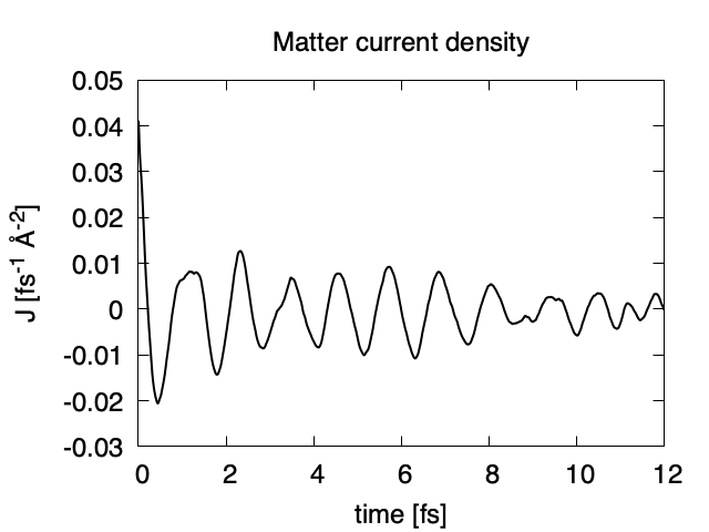
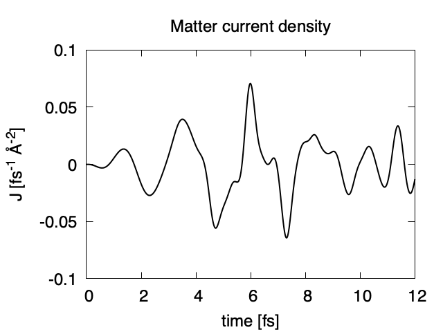
Using first column (time in femtosecond) and 16th column (matter current density in z direction), the following graph can be drawn.
Si_response.data
Time-frequency Fourier transformation of the macroscopic current density gives the conductivity of the system. The dielectric function is then calculated from the conductivity. They are stored in this file.
# Fourier-transform spectra:
# sigma: Conductivity
# eps: Dielectric constant
# 1:Energy[eV] 2:Re(sigma_x)[1/fs*V*Angstrom] 3:Re(sigma_y)[1/fs*V*Angstrom]
# 4:Re(sigma_z)[1/fs*V*Angstrom] 5:Im(sigma_x)[1/fs*V*Angstrom]
# 6:Im(sigma_y)[1/fs*V*Angstrom] 7:Im(sigma_z)[1/fs*V*Angstrom] 8:Re(eps_x)[none]
# 9:Re(eps_y)[none] 10:Re(eps_z)[none] 11:Im(eps_x)[none] 12:Im(eps_y)[none]
# 13:Im(eps_z)[none]
Using first column (energy in eV) and 10th (real part of the dielectric function) and 13th (imaginary part), we obtain the following graph.
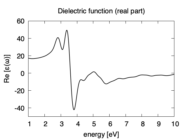
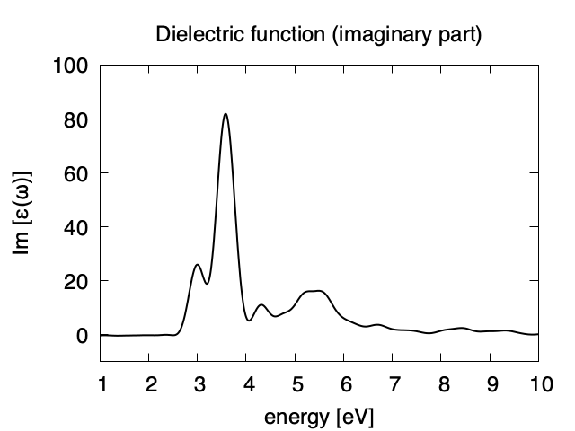
The imaginary part appears above the direct bandgap energy that is about 2.4 eV in the present calculation using local density approximation. Dielectric function below 1 eV are not accurate and and are not shown.
Si_rt_energy
Eall and Eall-Eall0 are total energy and electronic excitation energy, respectively.
# Real time calculation:
# Eall: Total energy
# Eall0: Initial energy
# 1:Time[fs] 2:Eall[eV] 3:Eall-Eall0[eV]
Exercise-6: Electron dynamics in crystalline silicon under a pulsed electric field
In this exercise, we learn the calculation of electron dynamics in crystalline silicon. A cubic unit cell that contains eight silicon atoms is used in the calculation. This exercise should be carried out after finishing the ground state calculation that was explained in Exercise-4.
In the calculation, a pulsed electric field specified by the following vector potential will be used,
\(A(t) = - \frac{E_0}{\omega} \hat z \cos^2 \frac{\pi}{T} \left( t - \frac{T}{2} \right) \sin \omega \left( t - \frac{T}{2} \right), \hspace{5mm} (0 < t < T).\)
The electric field is given by \(E(t) = -(1/c)(dA(t)/dt)\). The parameters that characterize the pulsed field such as the amplitude \(E_0\), frequency \(\omega\), pulse duration \(T\), polarization direction \(\hat z\), are specified in the input file. Time-dependent Kohn-Sham equation for Bloch orbitals are calculated in real time,
\(i\hbar \frac{\partial}{\partial t} u_{n{\bf k}}({\bf r},t) = H_{{\bf k} + (e/\hbar c){\bf A}(t)} u_{n{\bf k}}({\bf r},t).\)
Input files
To run the code, following files in samples are necessary:
| file name | description |
| Si_rt_pulse.inp | input file that contain input keywords and their values |
| Si_rps.dat | pseodupotential file for Carbon |
| restart | directory created in the ground
state calculation
(rename the directory from
data_for_restart to restart)
|
First two files are prepared in the directory SALMON/samples/exercise_06_bulkSi_rt/.
The file Si_rt_pulse.inp contains input keywords and their values.
The pseudoopotential file should be the same as that used in the ground state calculation.
In the directory restart, those files created in the ground state calculation
and stored in the directory data_for_restart are included.
Therefore, coopy the directory as cp -R data_for_restart restart
if you calculate at the same directory as you did the ground state calculation.
In the input file Si_rt_pulse.inp, input keywords are specified.
Most of them are mandatory to execute the electron dynamics calculation.
This will help you to prepare the input file for other systems that you want to calculate.
A complete list of the input keywords that can be used in the input file
can be found in List of input keywords.
!########################################################################################!
! Excercise 06: Electron dynamics in crystalline silicon under a pulsed electric field   !
!----------------------------------------------------------------------------------------!
! * The detail of this excercise is explained in our manual(see chapter: 'Exercises').   !
!   The manual can be obtained from: https://salmon-tddft.jp/documents.html              !
! * Input format consists of group of keywords like:                                     !
!     &group                                                                             !
!       input keyword = xxx                                                              !
!     /                                                                                  !
!   (see chapter: 'List of input keywords' in the manual)                                !
!----------------------------------------------------------------------------------------!
! * Conversion from unit_system = 'a.u.' to 'A_eV_fs':                                   !
!   Length: 1 [a.u.] = 0.52917721067    [Angstrom]                                       !
!   Energy: 1 [a.u.] = 27.21138505      [eV]                                             !
!   Time  : 1 [a.u.] = 0.02418884326505 [fs]                                             !
!----------------------------------------------------------------------------------------!
! * Copy the ground state data directory('data_for_restart') (or make symbolic link)     !
!   calculated in 'samples/exercise_04_bulkSi_gs/' and rename the directory to 'restart/'!
!   in the current directory.                                                            !
!########################################################################################!

&calculation
  !type of theory
  theory = 'tddft_pulse'
/
&control
  !common name of output files
  sysname = 'Si'
/
&units
  !units used in input and output files
  unit_system = 'A_eV_fs'
/
&system
  !periodic boundary condition
  yn_periodic = 'y'

  !grid box size(x,y,z)
  al(1:3) = 5.43d0, 5.43d0, 5.43d0

  !number of elements, atoms, electrons and states(bands)
  nelem  = 1
  natom  = 8
  nelec  = 32
  nstate = 32
/
&pseudo
  !name of input pseudo potential file
  file_pseudo(1) = './Si_rps.dat'

  !atomic number of element
  izatom(1) = 14

  !angular momentum of pseudopotential that will be treated as local
  lloc_ps(1) = 2
  !--- Caution -------------------------------------------!
  ! Index must correspond to those in &atomic_red_coor.   !
  !-------------------------------------------------------!
/
&functional
  !functional('PZ' is Perdew-Zunger LDA: Phys. Rev. B 23, 5048 (1981).)
  xc = 'PZ'
/
&rgrid
  !number of spatial grids(x,y,z)
  num_rgrid(1:3) = 12, 12, 12
/
&kgrid
  !number of k-points(x,y,z)
  num_kgrid(1:3) = 4, 4, 4
/
&tgrid
  !time step size and number of time grids(steps)
  dt = 0.002d0
  nt = 6000
/
&emfield
  !envelope shape of the incident pulse('Acos2': cos^2 type envelope for vector potential)
  ae_shape1 = 'Acos2'

  !peak intensity(W/cm^2) of the incident pulse
  I_wcm2_1 = 1.0d12

  !duration of the incident pulse
  tw1 = 10.672d0

  !mean photon energy(average frequency multiplied by the Planck constant) of the incident pulse
  omega1 = 1.55d0

  !polarization unit vector(real part) for the incident pulse(x,y,z)
  epdir_re1(1:3) = 0.0d0, 0.0d0, 1.0d0
  !--- Caution ---------------------------------------------------------!
  ! Definition of the incident pulse is written in:                     !
  ! https://www.sciencedirect.com/science/article/pii/S0010465518303412 !
  !---------------------------------------------------------------------!
/
&analysis
  !energy grid size and number of energy grids for output files
  de      = 0.01d0
  nenergy = 3000
/
&atomic_red_coor
  !cartesian atomic reduced coodinates
  'Si'       .0      .0      .0      1
  'Si'       .25     .25     .25     1
  'Si'       .5      .0      .5      1
  'Si'       .0      .5      .5      1
  'Si'       .5      .5      .0      1
  'Si'       .75     .25     .75     1
  'Si'       .25     .75     .75     1
  'Si'       .75     .75     .25     1
  !--- Format ---------------------------------------------------!
  ! 'symbol' x y z index(correspond to that of pseudo potential) !
  !--------------------------------------------------------------!
/
Execusion
In a multiprocess environment, calculation will be executed as:
$ mpiexec -n NPROC salmon < Si_rt_pulse.inp > Si_rt_pulse.out
where NPROC is the number of MPI processes. A standard output will be stored in the file Si_rt_pulse.out.
Output files
After the calculation, following output files are created in the directory that you run the code in addition to the standard output file,
| file name | description |
| Si_pulse.data | time-frequency Fourier transform of matter current and electric field |
| Si_rt.data | vector potential, electric field, and matter current as functions of time |
| Si_rt_energy | total energy and electronic excitation energy as functions of time |
| PS_Si_KY_n.dat | information on pseodupotential file for silicon atom |
We first explain the standard output file. In the beginning of the file, input variables used in the calculation are shown.
##############################################################################
# SALMON: Scalable Ab-initio Light-Matter simulator for Optics and Nanoscience
#
#                             Version 2.0.1
##############################################################################
  Libxc: [disabled]
   theory= tddft_pulse

 Total time step      =        6000
 Time step[fs]        =  2.000000000000000E-003
 Energy range         =        3000
 Energy resolution[eV]=  1.000000000000000E-002
Laser frequency     = 1.55[eV]
Pulse width of laser=     10.67200000[fs]
Laser intensity     =  0.10000000E+13[W/cm^2]
   use of real value orbitals =  F
 r-space parallelization: off
 ======
 ........
After that, the time evolution loop starts. At every 10 iterations, the time, current in three Cartesian directions, the number of electrons, and the total energy are displayed.
  time-step  time[fs]                               Current(xyz)[a.u.]      electrons Total energy[eV]
#----------------------------------------------------------------------
      10    0.02000000  0.11847131E-11 -0.47534543E-13 -0.43120486E-08    32.00000000     -850.76385276
      20    0.04000000  0.17733186E-11  0.12820952E-12 -0.33012195E-07    32.00000000     -850.76385276
      30    0.06000000  0.30965601E-11  0.23626542E-12 -0.10736819E-06    32.00000000     -850.76385275
      40    0.08000000  0.36612711E-11  0.47687574E-12 -0.24607217E-06    32.00000000     -850.76385272
      50    0.10000000  0.36958981E-11  0.62315158E-12 -0.46548014E-06    32.00000000     -850.76385263
      60    0.12000000  0.32186097E-11  0.11429104E-11 -0.77911390E-06    32.00000000     -850.76385239
      70    0.14000000  0.25712602E-11  0.15689467E-11 -0.11971541E-05    32.00000000     -850.76385186
      80    0.16000000  0.19447699E-11  0.18250920E-11 -0.17261976E-05    32.00000000     -850.76385082
      90    0.18000000  0.80514520E-12  0.18683828E-11 -0.23692381E-05    32.00000000     -850.76384896
Explanations of other output files are given below:
Si_rt.data
Results of time evolution calculation for vector potential, electric field, and matter current density.
# Real time calculation:
# Ac_ext: External vector potential field
# E_ext: External electric field
# Ac_tot: Total vector potential field
# E_tot: Total electric field
# Jm: Matter current density (electrons)
# 1:Time[fs] 2:Ac_ext_x[fs*V/Angstrom] 3:Ac_ext_y[fs*V/Angstrom] 4:Ac_ext_z[fs*V/Angstrom]
# 5:E_ext_x[V/Angstrom] 6:E_ext_y[V/Angstrom] 7:E_ext_z[V/Angstrom]
# 8:Ac_tot_x[fs*V/Angstrom] 9:Ac_tot_y[fs*V/Angstrom] 10:Ac_tot_z[fs*V/Angstrom]
# 11:E_tot_x[V/Angstrom] 12:E_tot_y[V/Angstrom] 13:E_tot_z[V/Angstrom]
# 14:Jm_x[1/fs*Angstrom^2] 15:Jm_y[1/fs*Angstrom^2] 16:Jm_z[1/fs*Angstrom^2]
The applied electric field is drawn using the first column (time in femtosecond) and the 7th column (electric field in z direction).

The matter current density is drawn using the first column (time in femtosecond) and 16th column (matter current density in z direction).
Si_pulse.data
Time-frequency Fourier transformation of the matter current and electric field.
# Fourier-transform spectra:
# energy: Frequency
# Jm: Matter current
# E_ext: External electric field
# E_tot: Total electric field
# 1:energy[eV] 2:Re(Jm_x)[1/Angstrom^2] 3:Re(Jm_y)[1/Angstrom^2] 4:Re(Jm_z)[1/Angstrom^2]
# 5:Im(Jm_x)[1/Angstrom^2] 6:Im(Jm_y)[1/Angstrom^2] 7:Im(Jm_z)[1/Angstrom^2]
# 8:|Jm_x|^2[1/Angstrom^4] 9:|Jm_y|^2[1/Angstrom^4] 10:|Jm_z|^2[1/Angstrom^4]
# 11:Re(E_ext_x)[fs*V/Angstrom] 12:Re(E_ext_y)[fs*V/Angstrom]
# 13:Re(E_ext_z)[fs*V/Angstrom] 14:Im(E_ext_x)[fs*V/Angstrom]
# 15:Im(E_ext_y)[fs*V/Angstrom] 16:Im(E_ext_z)[fs*V/Angstrom]
# 17:|E_ext_x|^2[fs^2*V^2/Angstrom^2] 18:|E_ext_y|^2[fs^2*V^2/Angstrom^2]
# 19:|E_ext_z|^2[fs^2*V^2/Angstrom^2] 20:Re(E_tot_x)[fs*V/Angstrom]
# 21:Re(E_tot_y)[fs*V/Angstrom] 22:Re(E_tot_z)[fs*V/Angstrom]
# 23:Im(E_tot_x)[fs*V/Angstrom] 24:Im(E_tot_y)[fs*V/Angstrom]
# 25:Im(E_tot_z)[fs*V/Angstrom] 26:|E_tot_x|^2[fs^2*V^2/Angstrom^2]
# 27:|E_tot_y|^2[fs^2*V^2/Angstrom^2] 28:|E_tot_z|^2[fs^2*V^2/Angstrom^2]
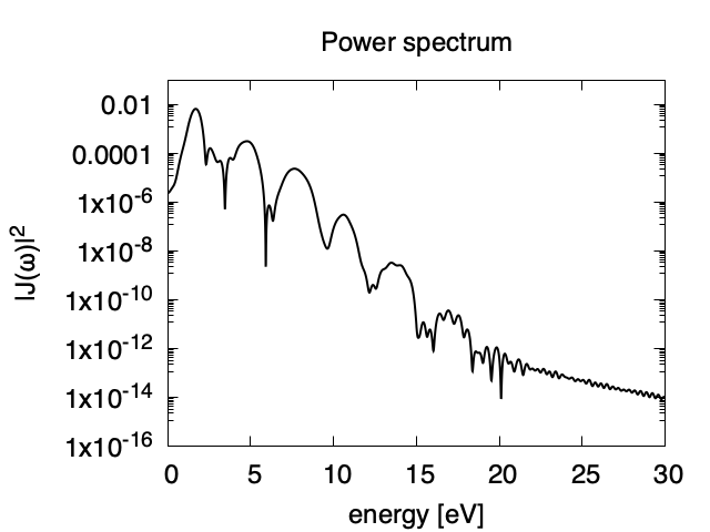
The power spectrum of the matter current density, \(|J(\omega)|^2\) is shown in logarithmic scale as a function of the energy, \(\hbar\omega\). High harmonic generations are visible in the spectrum.
Si_rt_energy
Energies are stored as functions of time.
# Real time calculation:
# Eall: Total energy
# Eall0: Initial energy
# 1:Time[a.u.] 2:Eall[a.u.] 3:Eall-Eall0[a.u.]
Eall and Eall-Eall0 are total energy and electronic excitation energy, respectively. The figure below shows the electronic excitation energy per unit cell volume as a function of time, using the first column (time in femtosecond) and the 3rd column (Eall-Eall0). Although the frequency is below the direct bandgap of silicon (2.4 eV in the LDA calculation), electronic excitations take place because of nonlinear absorption process.
Maxwell + TDDFT multiscale simulation
Exercise-7: Pulsed-light propagation through a silicon thin film
In this exercise, we learn the calculation of a propagation of pulsed light through a thin film of crystalline silicon. We consider an irradiation of a few-cycle, linearly polarized pulsed light normally on a thin film of 40 nm thickness. This exercise should be carried out after finishing the ground state calculation that was explained in Exercise-4.
In the calculation, macroscopic Maxwell equation that describes the light propagation and microscopic time-dependent Kohn-Sham equation that describes the electron dynamics are solved simultaneously. The light propagation is described by a one-dimensional light-propagation equation for the vector potential,
\(\frac{1}{c^2} \frac{\partial^2}{\partial X^2} A(X,t) - \frac{\partial^2}{\partial X^2} A(X,t) = \frac{4\pi}{c} I(X,t).\)
The direction of the propagation is set to x direction and the polarization of the pulse is set to z direction. The time profile of an incident pulse is given by
\(A(t) = - \frac{E_0}{\omega} \hat z \cos^2 \frac{\pi}{T} \left( t - \frac{T}{2} \right) \sin \omega \left( t - \frac{T}{2} \right), \hspace{5mm} (0 < t < T),\)
and is set in the vacuum region in front of the thin film. The parameters that characterize the pulsed field such as the amplitude \(E_0\), frequency \(\omega\), pulse duration \(T\) are specified in the input file.
To discribe the light propagation, macroscopic coordinate \(X\) is discretized as \(X_i\). At each grid point inside the silicon thin film, for which we take eight points \(i=1 \cdots 8\) in this exercise, time-dependent Kohn-Sham equation for Bloch orbitals are calculated in real time,
\(i\hbar \frac{\partial}{\partial t} u_{i n{\bf k}}({\bf r},t) = H_{{\bf k} + (e/\hbar c){\bf A}_i(t)} u_{i n{\bf k}}({\bf r},t).\)
From the Bloch orbital \(u_{in{\bf k}}({\bf r},t)\), we calculate the electric current \(I(X_i,t)\). We thus obtain a closed set of equations. Solving these equations simultaneously, we can describe macroscopic light propagation and microscopic electron dynamics at the same time.
Input files
To run the code, following files in samples are used:
| file name | description |
| Si_rt_multiscale.inp | input file that contain input keywords and their values. |
| Si_rps.dat | pseodupotential file for silicon |
| restart | directory created in the ground
state calculation
(rename the directory from
data_for_restart to restart)
|
First two files are prepared in the directory
SALMON/samples/exercise_07_bulkSi_multiscale/.
The file Si_rt_multiscale.inp contains input keywords and their values.
The pseudoopotential file should be the same as that used in the ground state calculation.
In the directory restart, those files created in the ground state calculation
and stored in the directory data_for_restart are included.
Therefore, coopy the directory as cp -R data_for_restart restart
if you calculate at the same directory as you did the ground state calculation.
In the input file Si_rt_multiscale.inp, input keywords are specified.
Most of them are mandatory to execute the electron dynamics calculation.
This will help you to prepare the input file for other systems that you want to calculate.
A complete list of the input keywords that can be used in the input file
can be found in List of input keywords.
!########################################################################################!
! Excercise 07: Maxwell+TDDFT multiscale simulation                                      !
!               (Pulsed-light propagation through a silicon thin film)                   !
!----------------------------------------------------------------------------------------!
! * The detail of this excercise is explained in our manual(see chapter: 'Exercises').   !
!   The manual can be obtained from: https://salmon-tddft.jp/documents.html              !
! * Input format consists of group of keywords like:                                     !
!     &group                                                                             !
!       input keyword = xxx                                                              !
!     /                                                                                  !
!   (see chapter: 'List of input keywords' in the manual)                                !
!----------------------------------------------------------------------------------------!
! * Conversion from unit_system = 'a.u.' to 'A_eV_fs':                                   !
!   Length: 1 [a.u.] = 0.52917721067    [Angstrom]                                       !
!   Energy: 1 [a.u.] = 27.21138505      [eV]                                             !
!   Time  : 1 [a.u.] = 0.02418884326505 [fs]                                             !
!----------------------------------------------------------------------------------------!
! * Copy the ground state data directory('data_for_restart') (or make symbolic link)     !
!   calculated in 'samples/exercise_04_bulkSi_gs/' and rename the directory to 'restart/'!
!   in the current directory.                                                            !
!########################################################################################!

&calculation
  !type of theory
  theory = 'multi_scale_maxwell_tddft'
/
&control
  !common name of output files
  sysname = 'Si'
/
&units
  !units used in input and output files
  unit_system = 'A_eV_fs'
/
&system
  !periodic boundary condition
  yn_periodic = 'y'

  !grid box size(x,y,z)
  al(1:3) = 5.43d0, 5.43d0, 5.43d0

  !number of elements, atoms, electrons and states(bands)
  nelem  = 1
  natom  = 8
  nelec  = 32
  nstate = 32
/
&pseudo
  !name of input pseudo potential file
  file_pseudo(1) = './Si_rps.dat'

  !atomic number of element
  izatom(1) = 14

  !angular momentum of pseudopotential that will be treated as local
  lloc_ps(1) = 2
  !--- Caution -------------------------------------------!
  ! Index must correspond to those in &atomic_red_coor.   !
  !-------------------------------------------------------!
/
&functional
  !functional('PZ' is Perdew-Zunger LDA: Phys. Rev. B 23, 5048 (1981).)
  xc = 'PZ'
/
&rgrid
  !number of spatial grids(x,y,z)
  num_rgrid(1:3) = 12, 12, 12
/
&kgrid
  !number of k-points(x,y,z)
  num_kgrid(1:3) = 4, 4, 4
/
&tgrid
  !time step size and number of time grids(steps)
  dt = 0.002d0
  nt = 8000
/
&emfield
  !envelope shape of the incident pulse('Acos2': cos^2 type envelope for vector potential)
  ae_shape1 = 'Acos2'

  !peak intensity(W/cm^2) of the incident pulse
  I_wcm2_1 = 1.0d12

  !duration of the incident pulse
  tw1 = 10.672d0

  !mean photon energy(average frequency multiplied by the Planck constant) of the incident pulse
  omega1 = 1.55d0

  !polarization unit vector(real part) for the incident pulse(x,y,z)
  epdir_re1(1:3) = 0.0d0, 0.0d0, 1.0d0
  !--- Caution ---------------------------------------------------------!
  ! Defenition of the incident pulse is written in:                     !
  ! https://www.sciencedirect.com/science/article/pii/S0010465518303412 !
  !---------------------------------------------------------------------!
/
&multiscale
  !number of macro grids in electromagnetic analysis for x, y, and z directions
  nx_m = 8
  ny_m = 1
  nz_m = 1

  !macro grid spacing for x, y, and z directions
  hx_m = 50.0d0
  hy_m = 50.0d0
  hz_m = 50.0d0

  !number of macroscopic grids for vacumm region
  !(nxvacl_m is for negative x-direction in front of material)
  !(nxvacr_m is for positive x-direction behind material)
  nxvacl_m = 1000
  nxvacr_m = 1000
/
&maxwell
  !boundary condition of electromagnetic analysis
  !first index(1-3 rows) corresponds to x, y, and z directions
  !second index(1-2 columns) corresponds to bottom and top of the directions
  !('abc' is absorbing boundary condition)
  boundary_em(1,1) = 'abc'
  boundary_em(1,2) = 'abc'
/
&atomic_red_coor
  !cartesian atomic reduced coodinates
  'Si'      .0      .0      .0      1
  'Si'      .25     .25     .25     1
  'Si'      .5      .0      .5      1
  'Si'      .0      .5      .5      1
  'Si'      .5      .5      .0      1
  'Si'      .75     .25     .75     1
  'Si'      .25     .75     .75     1
  'Si'      .75     .75     .25     1
  !--- Format ---------------------------------------------------!
  ! 'symbol' x y z index(correspond to that of pseudo potential) !
  !--------------------------------------------------------------!
/
Execusion
In a multiprocess environment, calculation will be executed as:
$ mpiexec -n NPROC salmon < Si_rt_multiscale.inp > Si_rt_multiscale.out
where NPROC is the number of MPI processes. A standard output will be stored in the file Si_rt_multiscale.out.
Output files
After the calculation, following output files and directories are created in the directory that you run the code in addition to the standard output file.
| file name | description |
| Si_m/mxxxxxx/Si_rt.data | vector potential, electric field,
and matter current
at macroscopic position xxxxxx
as functions of time
|
| Si_m/mxxxxxx/Si_rt_energy.data | total energy and electronic
excitation energy
at macroscopic position xxxxxx
as functions of time
|
| Si_m/mxxxxxx/PS_Si_KY_n.dat | information on pseodupotential
file for silicon atom
at macroscopic position xxxxxx
|
| Si_RT_Ac/Si_Ac_yyyyyy.data | vector potential,
electric field,
magnetic field,
electromagnetic current density
at time step yyyyyy
as function of spatial position
|
| Si_wave.data | waveform of incident, reflected, and transmitted waves |
We first explain the standard output file. In the beginning of the file, input variables used in the calculation are shown.
##############################################################################
# SALMON: Scalable Ab-initio Light-Matter simulator for Optics and Nanoscience
#
#                             Version 2.0.1
##############################################################################
  Libxc: [disabled]
   theory= multi_scale_maxwell_tddft
Initializing macropoint:     1-     8

 Total time step      =        8000
 Time step[fs]        =  2.000000000000000E-003
 Energy range         =        1000
 Energy resolution[eV]=  1.000000000000000E-002
Laser frequency     = 1.55[eV]
Pulse width of laser=     10.67200000[fs]
Laser intensity     =  0.10000000E+13[W/cm^2]
   use of real value orbitals =  F
 r-space parallelization: off
 ======
 .........
After that, the time evolution loop starts. At every 100 iterations, the step, grid point index, time, current in three Cartesian directions, the number of electrons, and the total energy are displayed.
   Step  Macro     Time                          Current      Electrons  Eabs/cell
                     fs                  1/fs*Angstrom^2                        eV
#------------------------------------------------------------------------------------------
    100      1    0.200  5.45E-010 -4.60E-011  2.70E-004    32.00000000  2.36E-006
    100      2    0.200  5.45E-010 -1.56E-011  1.83E-004    32.00000000  1.06E-006
    100      3    0.200  5.45E-010  7.19E-012  1.23E-004    32.00000000  4.62E-007
    100      4    0.200  5.45E-010  2.11E-011  8.14E-005    32.00000000  1.97E-007
    100      5    0.200  5.45E-010  2.11E-011  5.28E-005    32.00000000  8.04E-008
    100      6    0.200  5.45E-010  7.20E-012  3.34E-005    32.00000000  3.11E-008
    100      7    0.200  5.45E-010 -1.56E-011  2.03E-005    32.00000000  1.10E-008
    100      8    0.200  5.45E-010 -4.60E-011  1.13E-005    32.00000000  3.27E-009
    200      1    0.400  1.77E-011 -2.93E-013  9.70E-004    32.00000000  5.80E-005
    200      2    0.400  1.78E-011 -3.64E-011  7.50E-004    32.00000000  3.25E-005
    200      3    0.400  1.78E-011 -5.58E-011  5.75E-004    32.00000000  1.80E-005
    200      4    0.400  1.78E-011 -6.66E-011  4.38E-004    32.00000000  9.89E-006
Explanations of other output files are given below:
Si_wave.data
Waveforms of incident, reflected, and transmitted waves.
# 1D multiscale calculation:
# E_inc: E-field amplitude of incident wave
# E_ref: E-field amplitude of reflected wave
# E_tra: E-field amplitude of transmitted wave
# 1:Time[fs] 2:E_inc_x[V/Angstrom] 3:E_inc_y[V/Angstrom] 4:E_inc_z[V/Angstrom]
# 5:E_ref_x[V/Angstrom] 6:E_ref_y[V/Angstrom] 7:E_ref_z[V/Angstrom] 8:E_tra_x[V/Angstrom]
# 9:E_tra_y[V/Angstrom] 10:E_tra_z[V/Angstrom]
The figure below shows the incident, reflected, and transmitted electric fields that are drawn using the first column (time in femtosecond) and the 4th column (incident), 7th column (reflected), and 10th column (transmitted).
We find that the amplitude of the reflected pulse is comparable to the amplitude of the incudent pulse, while the phase is different by \(\pi\). The amplitude of the transmitted pulse is smaller than the incident pulse.
Si_m/mxxxxxx/Si_rt.data
The number xxxxxx in the directory name mxxxxxx specifies the position of macroscopic grid point. Vector potential, electric field, and matter current density as functions of time are included in the file.
# Real time calculation:
# Ac_ext: External vector potential field
# E_ext: External electric field
# Ac_tot: Total vector potential field
# E_tot: Total electric field
# Jm: Matter current density (electrons)
# 1:Time[fs] 2:Ac_ext_x[fs*V/Angstrom] 3:Ac_ext_y[fs*V/Angstrom] 4:Ac_ext_z[fs*V/Angstrom]
# 5:E_ext_x[V/Angstrom] 6:E_ext_y[V/Angstrom] 7:E_ext_z[V/Angstrom] 8:Ac_tot_x[fs*V/Angstrom]
# 9:Ac_tot_y[fs*V/Angstrom] 10:Ac_tot_z[fs*V/Angstrom] 11:E_tot_x[V/Angstrom]
# 12:E_tot_y[V/Angstrom] 13:E_tot_z[V/Angstrom]  14:Jm_x[1/fs*Angstrom^2]
# 15:Jm_y[1/fs*Angstrom^2] 16:Jm_z[1/fs*Angstrom^2]
The figure below shows the electric field at front and back surfaces.
Using 1st column (time in femtosecond) and 13th column (total electric field in z direction),
electric field at a macroscopic poisition inside the thin film can be plotted.
Using the file /m000001/Si_rt.data, electric field at the front surface is drawn
by red curve. Using the file /m000008/Si_rt.data, electric field at the back surface
is drawn by blue curve.
We find that the amplitude of the electric field at the front surface is small. It is consistent with the previous figure that showed incident and reflected pulses with a similar amplitude and opposite phase.
Si_m/mxxxxxx/Si_rt_energy.data
The number xxxxxx in the directory name mxxxxxx specifies the position of macroscopic grid point. Eall and Eall-Eall0 are total energy and electronic excitation energy, respectively.
# Real time calculation:
# Eall: Total energy
# Eall0: Initial energy
# 1:Time[fs] 2:Eall[eV] 3:Eall-Eall0[eV]
The figure below shows the electronic excitation energy per unit cell volume
at front and back surfaces using 1st columnn (time in femtosecond) and 3rd column
(Eall-Eall0).
Using the file /m000001/Si_rt_energy.data, the excitation energy at the
front surface is drawn by red curve. Using the file /m000008/Si_rt_energy.data,
the excitation energy at the back surface is drawn by blue curve.
The excitation energy is much larger at the back surface compared with the energy at the front surface. This is because the amplitude of the electric field at the back surface is larger than that of the front surface, as seen in the previous figure, and the excitation is a nonlinear process.
Si_RT_Ac/Si_Ac_yyyyyy.data
The number yyyyyy in the file name Si_Ac_yyyyyy.data specifies the time step.
Various quantities at the time step are included in the file as functions of macroscopic
position index.
# Multiscale TDDFT calculation
# IX, IY, IZ: FDTD Grid index
# x, y, z: Coordinates
# Ac: Vector potential field
# E: Electric field
# J_em: Electromagnetic current density
# 1:IX[none] 2:IY[none] 3:IZ[none] 4:Ac_x[fs*V/Angstrom] 5:Ac_y[fs*V/Angstrom]
# 6:Ac_z[fs*V/Angstrom] 7:E_x[V/Angstrom] 8:E_y[V/Angstrom] 9:E_z[V/Angstrom] 10:B_x[a.u.]
# 11:B_y[a.u.] 12:B_z[a.u.] 13:Jem_x[1/fs*Angstrom^2] 14:Jem_y[1/fs*Angstrom^2]
# 15:Jem_z[1/fs*Angstrom^2] 16:E_em[eV/vol] 17:E_abs[eV/vol]
The figure below shows spatial dependence of the electric field at three times, \(t=0\) fs (initial), \(t=8\) fs (pulse goes through the film), and \(t=16\) fs (final). It is drawn using the first column multiplied by the step size of \(X\) and 9th column (electric field).
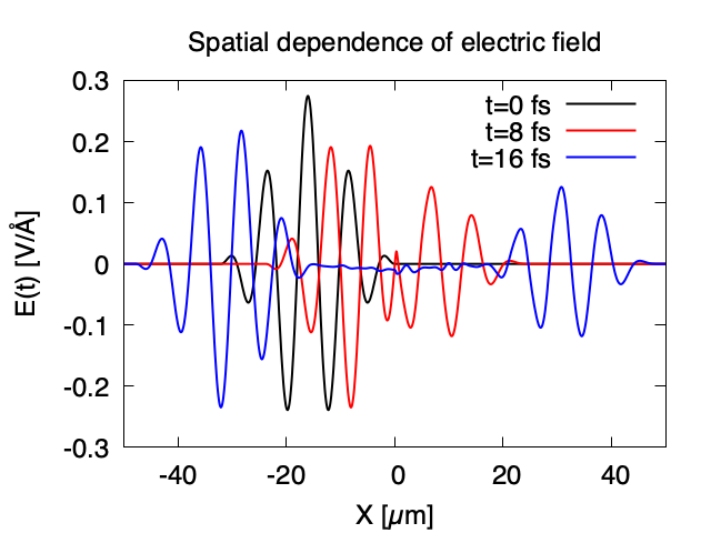
Geometry optimization and Ehrenfest molecular dynamics
Exercise-8: Geometry optimization of C2H2 molecule
In this exercise, we learn the calculation of geometry optimization of acetylene (C2H2) molecule, solving the static Kohn-Sham equation. This exercise will be useful to learn how to set up calculations in SALMON for any isolated systems such as molecules and nanoparticles.
Input files
To run the code, following files in samples are used:
| file name | description |
| C2H2_opt.inp | input file that contains input keywords and their values |
| C_rps.dat | pseodupotential file for carbon atom |
| H_rps.dat | pseudopotential file for hydrogen atom |
In the input file C2H2_opt.inp, input keywords are specified.
Most of them are mandatory to execute the geometry optimization.
This will help you to prepare an input file for other systems that you
want to calculate. A complete list of the input keywords that can be
used in the input file can be found in
List of input keywords.
!########################################################################################!
! Excercise 08: Geometry optimization of C2H2 molecule                                   !
!----------------------------------------------------------------------------------------!
! * The detail of this excercise is expained in our manual(see chapter: 'Exercises').    !
!   The manual can be obtained from: https://salmon-tddft.jp/documents.html              !
! * Input format consists of group of keywords like:                                     !
!     &group                                                                             !
!       input keyword = xxx                                                              !
!     /                                                                                  !
!   (see chapter: 'List of input keywords' in the manual)                                !
!----------------------------------------------------------------------------------------!
! * Conversion from unit_system = 'a.u.' to 'A_eV_fs':                                   !
!   Length: 1 [a.u.] = 0.52917721067    [Angstrom]                                       !
!   Energy: 1 [a.u.] = 27.21138505      [eV]                                             !
!   Time  : 1 [a.u.] = 0.02418884326505 [fs]                                             !
!########################################################################################!

&calculation
  !type of theory
  theory = 'dft'

  !geometry optimization option
  yn_opt = 'y'
/
&control
  !common name of output files
  sysname = 'C2H2'
/
&units
  !units used in input and output files
  unit_system = 'A_eV_fs'
/
&system
  !periodic boundary condition
  yn_periodic = 'n'

  !grid box size(x,y,z)
  al(1:3) = 12.0d0, 12.0d0, 16.0d0

  !number of elements, atoms, electrons and states(orbitals)
  nelem  = 2
  natom  = 4
  nelec  = 10
  nstate = 6
/
&pseudo
  !name of input pseudo potential file
  file_pseudo(1) = './C_rps.dat'
  file_pseudo(2) = './H_rps.dat'

  !atomic number of element
  izatom(1) = 6
  izatom(2) = 1

  !angular momentum of pseudopotential that will be treated as local
  lloc_ps(1) = 1
  lloc_ps(2) = 0
  !--- Caution ---------------------------------------!
  ! Indices must correspond to those in &atomic_coor. !
  !---------------------------------------------------!
/
&functional
  !functional('PZ' is Perdew-Zunger LDA: Phys. Rev. B 23, 5048 (1981).)
  xc = 'PZ'
/
&rgrid
  !spatial grid spacing(x,y,z)
  dl(1:3) = 0.20d0, 0.20d, 0.20d0
/
&scf
  !maximum number of scf iteration and threshold of convergence for ground state calculation
  nscf      = 300
  threshold = 1.0d-9
/
&opt
  !threshold(maximum force on atom) of convergence for geometry optimization
  convrg_opt_fmax = 1.0d-3
/

&atomic_coor
  !cartesian atomic coodinates
  'C'    0.0    0.0    0.6  1  y
  'H'    0.0    0.0    1.7  2  y
  'C'    0.0    0.0   -0.6  1  y
  'H'    0.0    0.0   -1.7  2  y
  !--- Format -------------------------------------------------------!
  ! 'symbol' x y z index(correspond to that of pseudo potential) y/n !
  !--- Caution ------------------------------------------------------!
  ! final index(y/n) determines free/fix for the atom coordinate.    !
  !------------------------------------------------------------------!
/
Output files
After the calculation, following output files and a directory are created in the directory that you run the code,
| name | description |
| C2H2_info.data | information on ground state solution |
| C2H2_eigen.data | 1 particle energies |
| C2H2_trj.xyz | atomic coordinates during the geometry optimization |
| C2H2_k.data | k-point distribution (for isolated systems, only gamma point is described) |
| data_for_restart | directory where files used in the real-time calculation are contained |
| PS_C_KY_n.dat | information on pseodupotential file for carbon atom |
| PS_H_KY_n.dat | information on pseodupotential file for hydrogen atom |
data_for_restart) from:Main results of the calculation such as orbital energies are included in C2H2_info.data.
Explanations of the C2H2_info.data and other output files are below:
C2H2_info.data
Calculated orbital and total energies as well as parameters specified in the input file are shown in this file.
C2H2_eigen.data
1 particle energies.
#esp: single-particle energies (eigen energies)
#occ: occupation numbers, io: orbital index
# 1:io, 2:esp[eV], 3:occ
C2H2_trj.xyz
The atomic coordinates during the geometry optimization in xyz format.
C2H2_k.data
k-point distribution(for isolated systems, only gamma point is described).
# ik: k-point index
# kx,ky,kz: Reduced coordinate of k-points
# wk: Weight of k-point
# 1:ik[none] 2:kx[none] 3:ky[none] 4:kz[none] 5:wk[none]
# coefficients (2*pi/a [a.u.]) in kx, ky, kz
Exercise-9: Ehrenfest molecular dynamics of C2H2 molecule
In this exercise, we learn the calculation of the molecular dynamics in the acetylene (C2H2) molecule under a pulsed electric field, solving the time-dependent Kohn-Sham equation and the Newtonian equation. As outputs of the calculation, time-evolution of the electron density as well as molecular structures and associated quantities such as the electron and ion kinetic energies, the electric dipole moment of the system and temperature as functions of time are calculated.. This tutorial should be carried out after finishing the geometry optimization that was explained in Exercise-8. In the calculation, a pulsed electric field that has \(\cos^2\) envelope shape is applied. The parameters that characterize the pulsed field such as magnitude, frequency, polarization direction, and carrier envelope phase are specified in the input file.
Input files
To run the code, following files in samples are used.
The directory restart is created in the ground state calculation as data_for_restart.
Pseudopotential files are already used in the geometry optimization.
Therefore, C2H2_md.inp that specifies input keywords and their values
for the pulsed electric field and molecular dynamics calculations
is the only file that the users need to prepare.
| file name | description |
| C2H2_md.inp | input file that contain input keywords and their values. |
| C_rps.dat | pseodupotential file for carbon |
| H_rps.dat | pseudopotential file for hydrogen |
| restart | directory created in the geometry
optimization
(rename the directory from
data_for_restart to restart)
|
In the input file C2H2_md.inp, input keywords are specified.
Most of them are mandatory to execute the calculation of
electron dynamics induced by a pulsed electric field.
This will help you to prepare the input file for other systems and other
pulsed electric fields with molecular dynamics calculation that you want to calculate.
A complete list of the input keywords that can be used in the input file can be found in
List of input keywords.
!########################################################################################!
! Excercise 09: Ehrenfest molecular dynamics of C2H2 molecule                            !
!----------------------------------------------------------------------------------------!
! * The detail of this excercise is expained in our manual(see chapter: 'Exercises').    !
!   The manual can be obtained from: https://salmon-tddft.jp/documents.html              !
! * Input format consists of group of keywords like:                                     !
!     &group                                                                             !
!       input keyword = xxx                                                              !
!     /                                                                                  !
!   (see chapter: 'List of input keywords' in the manual)                                !
!----------------------------------------------------------------------------------------!
! * Conversion from unit_system = 'a.u.' to 'A_eV_fs':                                   !
!   Length: 1 [a.u.] = 0.52917721067    [Angstrom]                                       !
!   Energy: 1 [a.u.] = 27.21138505      [eV]                                             !
!   Time  : 1 [a.u.] = 0.02418884326505 [fs]                                             !
!----------------------------------------------------------------------------------------!
! * Ehrenfest-MD option is still trial.                                                  !
! * Copy the ground state data directory ('data_for_restart') (or make symbolic link)    !
!   calculated in 'samples/exercise_08_C2H2_opt/' and rename the directory to 'restart/' !
!   in the current directory.                                                            !
!########################################################################################!

&calculation
  !type of theory
  theory = 'tddft_pulse'

  !molecular dynamics option
  yn_md  = 'y'
/
&control
  !common name of output files
  sysname = 'C2H2'
/
&units
  !units used in input and output files
  unit_system = 'A_eV_fs'
/
&system
  !periodic boundary condition
  yn_periodic = 'n'

  !grid box size(x,y,z)
  al(1:3) = 12.0d0, 12.0d0, 16.0d0

  !number of elements, atoms, electrons and states(orbitals)
  nelem  = 2
  natom  = 4
  nelec  = 10
  nstate = 6
/
&pseudo
  !name of input pseudo potential file
  file_pseudo(1) = './C_rps.dat'
  file_pseudo(2) = './H_rps.dat'

  !atomic number of element
  izatom(1) = 6
  izatom(2) = 1

  !angular momentum of pseudopotential that will be treated as local
  lloc_ps(1) = 1
  lloc_ps(2) = 0
  !--- Caution ---------------------------------------!
  ! Indices must correspond to those in &atomic_coor. !
  !---------------------------------------------------!
/
&functional
  !functional('PZ' is Perdew-Zunger LDA: Phys. Rev. B 23, 5048 (1981).)
  xc = 'PZ'
/
&rgrid
  !spatial grid spacing(x,y,z)
  dl(1:3) = 0.20d0, 0.20d0, 0.20d0
/
&tgrid
  !time step size and number of time grids(steps)
  dt = 1.00d-3
  nt = 5000
/
&emfield
  !envelope shape of the incident pulse('Ecos2': cos^2 type envelope for scalar potential)
  ae_shape1 = 'Ecos2'

  !peak intensity(W/cm^2) of the incident pulse
  I_wcm2_1 = 1.00d8

  !duration of the incident pulse
  tw1 = 6.00d0

  !mean photon energy(average frequency multiplied by the Planck constant) of the incident pulse
  omega1 = 9.28d0

  !polarization unit vector(real part) for the incident pulse(x,y,z)
  epdir_re1(1:3) = 0.00d0, 0.00d0, 1.00d0

  !carrier emvelope phase of the incident pulse
  !(phi_cep1 must be 0.25 + 0.5 * n(integer) when ae_shape1 = 'Ecos2')
  phi_cep1 = 0.75d0
  !--- Caution ---------------------------------------------------------!
  ! Defenition of the incident pulse is wrriten in:                     !
  ! https://www.sciencedirect.com/science/article/pii/S0010465518303412 !
  !---------------------------------------------------------------------!
/
&md
  !ensemble
  ensemble = 'NVE'

  !set of initial velocities
  yn_set_ini_velocity = 'y'

  !setting temperature [K] for NVT ensemble, velocity scaling,
  !and generating initial velocities
  temperature0_ion_k = 300.0d0

  !time step interval for updating pseudopotential
  step_update_ps = 20
/
Output files
After the calculation, following output files are created in the directory that you run the code,
| file name | description |
| C2H2_pulse.data | dipole moment as functions of energy |
| C2H2_rt.data | components of
change of dipole moment
(electrons/plus definition)
and total dipole moment
(electrons/minus + ions/plus)
as functions of time
|
| C2H2_rt_energy.data | components of total energy and difference of total energy as functions of time |
| C2H2_trj.xyz | Trajectory of atoms(ions): Atomic coordinates, velocities, and forces are printed |
| PS_C_KY_n.dat | information on pseodupotential file for carbon atom |
| PS_H_KY_n.dat | information on pseodupotential file for hydrogen atom |
Explanations of the files are described below:
C2H2_pulse.data
Time-frequency Fourier transformation of the dipole moment.
# Fourier-transform spectra:
# energy: Frequency
# dm: Dopile moment
# 1:energy[eV] 2:Re(dm_x)[fs*Angstrom] 3:Re(dm_y)[fs*Angstrom] 4:Re(dm_z)[fs*Angstrom] 5:Im(dm_x)[fs*Angstrom] 6:Im(dm_y)[fs*Angstrom] 7:Im(dm_z)[fs*Angstrom] 8:|dm_x|^2[fs^2*Angstrom^2] 9:|dm_y|^2[fs^2*Angstrom^2] 10:|dm_z|^2[fs^2*Angstrom^2]
C2H2_rt.data
Results of time evolution calculation for vector potential, electric field, and dipole moment.
# Real time calculation:
# Ac_ext: External vector potential field
# E_ext: External electric field
# Ac_tot: Total vector potential field
# E_tot: Total electric field
# ddm_e: Change of dipole moment (electrons/plus definition)
# dm: Total dipole moment (electrons/minus + ions/plus)
# 1:Time[fs] 2:Ac_ext_x[fs*V/Angstrom] 3:Ac_ext_y[fs*V/Angstrom] 4:Ac_ext_z[fs*V/Angstrom] 5:E_ext_x[V/Angstrom] 6:E_ext_y[V/Angstrom] 7:E_ext_z[V/Angstrom] 8:Ac_tot_x[fs*V/Angstrom] 9:Ac_tot_y[fs*V/Angstrom] 10:Ac_tot_z[fs*V/Angstrom] 11:E_tot_x[V/Angstrom] 12:E_tot_y[V/Angstrom] 13:E_tot_z[V/Angstrom] 14:ddm_e_x[Angstrom] 15:ddm_e_y[Angstrom] 16:ddm_e_z[Angstrom] 17:dm_x[Angstrom] 18:dm_y[Angstrom] 19:dm_z[Angstrom]
C2H2_rt_energy.data
Eall and Eall-Eall0 are total energy and electronic excitation energy, respectively.
# Real time calculation:
# Eall: Total energy
# Eall0: Initial energy
# Tion: Kinetic energy of ions
# Temperature_ion: Temperature of ions
# E_work: Work energy of ions(sum f*dr)
# 1:Time[fs] 2:Eall[eV] 3:Eall-Eall0[eV] # 4:Tion[eV] 5:Temperature_ion[K] 6:E_work[eV]
C2H2_trj.xyz
Atomic coordinates [Angstrom], velocities [a.u.] and forces [a.u.] are printed along the time evolution in xyz format.
FDTD simulation(electromagnetic analysis)
Exercise-10: Absorption-, Scattering-, and Extinction-cross-sections of an Au nanoparticle in FDTD simulation
In this exercise, we learn the calculation of the absorption-, scattering-, and extinction-cross-sections of an Au nanoparticle, by applying the incident pulse in the time-dependent Maxwell equations. As outputs of the calculation, those cross-sections and the time response of the electromagnetic field are calculated. A pulsed electric field that has \(\cos^2\) envelope shape is applied. The parameters that characterize the pulsed field such as magnitude, frequency, polarization direction, and carrier envelope phase are specified in the input file.
Input files
To run the code, the input file AuNP_fdtd.inp is used:
| file name | description |
| AuNP_fdtd.inp | input file that contains input keywords and their values. |
In the input file AuNP_fdtd.inp, input keywords are specified.
Most of them are mandatory to execute this exercise.
This will help you to prepare the input file for other systems that you want to calculate.
A complete list of the input keywords that can be used in the input file
can be found in List of input keywords.
!########################################################################################!
! Excercise 10: Absorption-, Scattering-, and Extinction-cross-sections                  !
!               of an Au nanoparticle in FDTD simulation                                 !
!----------------------------------------------------------------------------------------!
! * The detail of this excercise is explained in our manual(see chapter: 'Exercises').   !
!   The manual can be obtained from: https://salmon-tddft.jp/documents.html              !
! * Input format consists of group of keywords like:                                     !
!     &group                                                                             !
!       input keyword = xxx                                                              !
!     /                                                                                  !
!   (see chapter: 'List of input keywords' in the manual)                                !
!----------------------------------------------------------------------------------------!
! * Conversion from unit_system = 'a.u.' to 'A_eV_fs':                                   !
!   Length: 1 [a.u.] = 0.52917721067    [Angstrom]                                       !
!   Energy: 1 [a.u.] = 27.21138505      [eV]                                             !
!   Time  : 1 [a.u.] = 0.02418884326505 [fs]                                             !
!########################################################################################!

&calculation
  !type of theory
  theory = 'maxwell'
/
&control
  !common name of output files
  sysname = 'AuNP'

  !name of directory where output files are contained
  base_directory = 'result'
/
&units
  !units used in input and output files
  unit_system = 'A_eV_fs'
/
&system
  !periodic boundary condition
  yn_periodic = 'n'
/
&emfield
  !envelope shape of the incident pulse('Ecos2': cos^2 type envelope for scalar potential)
  ae_shape1 = 'Ecos2'

  !peak intensity(W/cm^2) of the incident pulse
  I_wcm2_1 = 1.00d6

  !duration of the incident pulse
  tw1 = 7.50d0

  !mean photon energy(average frequency multiplied by the Planck constant) of the incident pulse
  omega1 = 2.30d0

  !polarization unit vector(real part) for the incident pulse(x,y,z)
  epdir_re1(1:3) = 1.00d0, 0.00d0, 0.00d0

  !carrier emvelope phase of the incident pulse
  !(phi_cep1 must be 0.25 + 0.5 * n(integer) when ae_shape1 = 'Ecos2')
  phi_cep1 = 0.75d0
  !--- Caution ---------------------------------------------------------!
  ! Definition of the incident pulse is written in:                     !
  ! https://www.sciencedirect.com/science/article/pii/S0010465518303412 !
  !---------------------------------------------------------------------!
/
&maxwell
  !grid box size(x,y,z) and number of spatial grids(x,y,z)
  al_em(1:3)        = 600.0d1, 600.0d1, 600.0d1
  num_rgrid_em(1:3) = 100, 100, 100
  !--- Caution ---------------------------------------------------------!
  ! Copumutational domain is set as:                                    !
  !         -al_em/2 ~ al_em/2 for yn_periodic='n'                      !
  ! whereas        0 ~ al_em   for yn_periodic='y'.                     !
  !---------------------------------------------------------------------!

  !total time
  at_em = 50.0d0
  !--- TIPS ------------------------------------------------------------!
  ! Two of at_em, dt_em, and nt_em must be set.                         !
  ! Otherwise, both at_em and nt_em or either of those must be set.     !
  ! The latter automatically determines dt_em from CFL condition.       !
  !---------------------------------------------------------------------!

  !*** SHAPE INFORMATION(START) ****************************************!
  !make and output shape file
  yn_make_shape   = 'y'
  yn_output_shape = 'y'

  !number of shape-template
  n_s = 1

  !media ID and type of shape-template(shape ID)
  id_s(1)  = 1
  typ_s(1) = 'ellipsoid'

  !information and origin of shape-template:
  !inf_s(shape ID,x-diameter,y-diameter,z-diameter)
  !ori_s(shape ID,x,y,z)
  inf_s(1,1:3) = 200.0d1, 200.0d1, 200.0d1
  ori_s(1,1:3) = 0.000d1, 0.000d1, 0.000d1
  !--- TIPS ------------------------------------------------------------!
  ! * shape file can be generated by also an external program           !
  !   'FDTD_make_shape' in SALMON utilities                             !
  !   (https://salmon-tddft.jp/utilities.html).                         !
  !   The generated shape file can be read by an input keyword          !
  !   'shape_file' in &maxwell.                                         !
  ! * More complex shapes can be generated by other input keywords      !
  !   which are in common with those used in 'FDTD_make_shape'.         !
  !---------------------------------------------------------------------!
  !*** SHAPE INFORMATION(END) ******************************************!

  !*** MEDIA INFORMATION(START) ****************************************!
  !number and type of media(media ID)
  media_num     = 1
  media_type(1) = 'lorentz-drude'
  !--- Au described by Lorentz-Drude model -----------------------------!
  ! The parameters are determined from:                                 !
  ! (https://doi.org/10.1364/AO.37.005271)                              !
  !---------------------------------------------------------------------!

  !number of poles and plasma frequency of LD media(media ID)
  pole_num_ld(1) = 6
  omega_p_ld(1)  = 9.030d0

  !oscillator strength, collision frequency,
  !and oscillator frequency of LD media(media ID,pole ID)
  f_ld(1,1:6)     = 0.760d0, 0.024d0, 0.010d0, 0.071d0, 0.601d0, 4.384d0
  gamma_ld(1,1:6) = 0.053d0, 0.241d0, 0.345d0, 0.870d0, 2.494d0, 2.214d0
  omega_ld(1,1:6) = 0.000d0, 0.415d0, 0.830d0, 2.969d0, 4.304d0, 13.32d0
  !--- TIPS ------------------------------------------------------------!
  ! If you calclate a metallic nanoparticle surrounded by something     !
  ! other than vacuum/air, such as Au nanoparticle in water solution,   !
  ! you should change 'epsilon_em(0)' in &maxwell,                      !
  ! which specifies the permittivity of surrounding medium.             !
  !---------------------------------------------------------------------!
  !*** MEDIA INFORMATION(END) ******************************************!

  !*** SOURCE INFORMATION(START) ***************************************!
  !type of method to generate the incident pulse
  !('source': incident current source)
  wave_input = 'source'

  !location of source(x,y,z)
  source_loc1(1:3) = 0.000d1, 0.000d1, -200.0d1

  !propagation direction of the incident pulse(x,y,z)
  ek_dir1(1:3) = 0.000d0, 0.000d0, 1.000d0
  !*** SOURCE INFORMATION(END) *****************************************!

  !*** ASE INFORMATION(START) ******************************************!
  !number of wavelength grid points
  !for Absorption-, Scattering-, and Extinction-cross-sections(ASE)
  !normalized by the spectral distribution of the incident pulse
  ase_num_em = 100

  !minimum and maximum values of wavelength for ASE
  ase_wav_min_em = 400.0d1
  ase_wav_max_em = 800.0d1
  !--- TIPS ------------------------------------------------------------!
  ! ase_ene_min_em and ase_wav_max_em can also be available.            !
  ! If those are used, ASE are outputed for energy axis.                !
  !---------------------------------------------------------------------!

  !size of a closed surface (box shape) to calculate ASE(x-size,y-size,z-size)
  ase_box_size_em(1:3) = 300.0d1, 300.0d1, 300.0d1
  !*** ASE INFORMATION(END) *********************************************!

  !*** OBSERVATION INFORMATION(START) ***********************************!
  !number of observation points
  obs_num_em = 1

  !location of observation point(observation ID,x,y,z)
  obs_loc_em(1,1:3) = 0.0d0, 0.0d0, 0.0d0
  !--- TIPS ------------------------------------------------------------!
  ! * If you specify yn_obs_plane_em(1) = 'y',                          !
  !   animation files can be made by an external program                !
  !   'FDTD_make_figani' in SALMON utilities.                           !
  !   (https://salmon-tddft.jp/utilities.html).                         !
  !   The animation file visualizes electromagnetic field distributions !
  !   on the cross-section including the observation point              !
  !   whose location is determined by obs_loc_em.                       !
  ! * If you specify obs_plane_ene_em(1,1:n) by certain values          !
  !   space-energy distribution of electromagnetic field is outputed    !
  !---------------------------------------------------------------------!
  !*** OBSERVATION INFORMATION(END) ************************************!
/
FDTD_make_shape in SALMON utilities (https://salmon-tddft.jp/utilities.html).Output files
After the calculation, following output files are created in the directory result,
| file name | description |
| AuNP_ase_with_wf.data | A-, S-, and E-corss-sections as functions of wavelength, where window function is applied in Fourier transformation |
| AuNP_ase_without_wf.data | A-, S-, and E-corss-sections as functions of wavelength, where window function is not applied in Fourier transformation |
| obs1_at_point_rt.data | components of electric and magnetic fields as functions of time |
| shape.cube | shape file for fdtd |
Explanations of the files are described below:
AuNP_ase_with_wf.data
Results of A-, S-, and E-cross-sections normalized by the spectral distribution of the incident pulse. Also the spectral distribution for pointing vector of incident pulse is included. Window function is applied in Fourier transformation.
# Absorption-, Scattering-, and Extinction-cross-sections normalized by the spectral distribution of the incident pulse (with window function):
# sigma_a: Absorption cross-section
# sigma_s: Scattering cross-section
# sigma_e: Extinction cross-section
# S: Pointing vector of incident pulse along propagation direction
# 1:Wavelength[Angstrom] 2:sigma_a[Angstrom^2] 3:sigma_s[Angstrom^2] 4:sigma_e[Angstrom^2] 5:S[VA/Angstrom^2*fs^2]
AuNP_ase_without_wf.data
Results of A-, S-, and E-cross-sections normalized by the spectral distribution of the incident pulse. Also the spectral distribution for pointing vector of incident pulse is included. Window function is not applied in Fourier transformation.
# Absorption-, Scattering-, and Extinction-cross-sections normalized by the spectral distribution of the incident pulse (without window function):
# sigma_a: Absorption cross-section
# sigma_s: Scattering cross-section
# sigma_e: Extinction cross-section
# S: Pointing vector of incident pulse along propagation direction
# 1:Wavelength[Angstrom] 2:sigma_a[Angstrom^2] 3:sigma_s[Angstrom^2] 4:sigma_e[Angstrom^2] 5:S[VA/Angstrom^2*fs^2]
obs0_info.data
This file is used to generate animation files by using SALMON utilities with yn_obs_plane_em: https://salmon-tddft.jp/utilities.html
obs1_at_point_rt.data
Results of time evolution calculation for electric and magnetic fields at observation point 1.
# Real time calculation:
# E: Electric field
# H: Magnetic field
# 1:Time[fs] 2:E_x[V/Angstrom] 3:E_y[V/Angstrom] 4:E_z[V/Angstrom] 5:H_x[A/Angstrom] 6:H_y[A/Angstrom] 7:H_z[A/Angstrom]
shape.cube
Shape file generated by yn_make_shape.
Exercise-11: Absorption-, Reflection-, and Transmission-rates of an Au nanoparticles metasurface in FDTD simulation
In this exercise, we learn the calculation ofthe absorption-, reflection-, and transmission-rates of a metasurface, in which Au nanoparticles are periodically arrayed in two-dimension, by applying the incident pulse in the time-dependent Maxwell equations. As outputs of the calculation, those rates and the time response of the electromagnetic field are calculated. A pulsed electric field that has \(\cos^2\) envelope shape is applied. The parameters that characterize the pulsed field such as magnitude, frequency, polarization direction, and carrier envelope phase are specified in the input file.
Input files
To run the code, the input file AuNP_fdtd.inp is used:
| file name | description |
| AuNPs_fdtd.inp | input file that contains input keywords and their values. |
In the input file AuNPs_fdtd.inp, input keywords are specified.
Most of them are mandatory to execute this exercise.
This will help you to prepare the input file for other systems that you want to calculate.
A complete list of the input keywords that can be used in the input file
can be found in List of input keywords.
!########################################################################################!
! Excercise 11: Absorption-, Reflection-, and Transmission-rates                         !
!               of an Au nanoparticles metasurface in FDTD simulation                    !
!----------------------------------------------------------------------------------------!
! * The detail of this excercise is explained in our manual(see chapter: 'Exercises').   !
!   The manual can be obtained from: https://salmon-tddft.jp/documents.html              !
! * Input format consists of group of keywords like:                                     !
!     &group                                                                             !
!       input keyword = xxx                                                              !
!     /                                                                                  !
!   (see chapter: 'List of input keywords' in the manual)                                !
!----------------------------------------------------------------------------------------!
! * Conversion from unit_system = 'a.u.' to 'A_eV_fs':                                   !
!   Length: 1 [a.u.] = 0.52917721067    [Angstrom]                                       !
!   Energy: 1 [a.u.] = 27.21138505      [eV]                                             !
!   Time  : 1 [a.u.] = 0.02418884326505 [fs]                                             !
!########################################################################################!

&calculation
  !type of theory
  theory = 'maxwell'
/
&control
  !common name of output files
  sysname = 'AuNPs'

  !name of directory where output files are contained
  base_directory = 'result'
/
&units
  !units used in input and output files
  unit_system = 'A_eV_fs'
/
&system
  !periodic boundary condition
  yn_periodic = 'y'
/
&emfield
  !envelope shape of the incident pulse('Ecos2': cos^2 type envelope for scalar potential)
  ae_shape1 = 'Ecos2'

  !peak intensity(W/cm^2) of the incident pulse
  I_wcm2_1 = 1.00d6

  !duration of the incident pulse
  tw1 = 7.50d0

  !mean photon energy(average frequency multiplied by the Planck constant) of the incident pulse
  omega1 = 2.30d0

  !polarization unit vector(real part) for the incident pulse(x,y,z)
  epdir_re1(1:3) = 1.00d0, 0.00d0, 0.00d0

  !carrier emvelope phase of the incident pulse
  !(phi_cep1 must be 0.25 + 0.5 * n(integer) when ae_shape1 = 'Ecos2')
  phi_cep1 = 0.75d0
  !--- Caution ---------------------------------------------------------!
  ! Definition of the incident pulse is written in:                     !
  ! https://www.sciencedirect.com/science/article/pii/S0010465518303412 !
  !---------------------------------------------------------------------!
/
&maxwell
  !grid box size(x,y,z) and number of spatial grids(x,y,z)
  al_em(1:3)        = 300.0d1, 300.0d1, 600.0d1
  num_rgrid_em(1:3) = 50, 50, 100
  !--- Caution ---------------------------------------------------------!
  ! Copumutational domain is set as:                                    !
  !         -al_em/2 ~ al_em/2 for yn_periodic='n'                      !
  ! whereas        0 ~ al_em   for yn_periodic='y'.                     !
  !---------------------------------------------------------------------!

  !total time
  at_em = 50.0d0
  !--- TIPS ------------------------------------------------------------!
  ! Two of at_em, dt_em, and nt_em must be set.                         !
  ! Otherwise, both at_em and nt_em or either of those must be set.     !
  ! The latter automatically determines dt_em from CFL condition.       !
  !---------------------------------------------------------------------!

  !absorbing boudnary conditions at bottom and top on z axis
  boundary_em(3,1) = 'abc'
  boundary_em(3,2) = 'abc'

  !*** SHAPE INFORMATION(START) ****************************************!
  !make and output shape file
  yn_make_shape   = 'y'
  yn_output_shape = 'y'

  !number of shape-template
  n_s = 1

  !media ID and type of shape-template(shape ID)
  id_s(1)  = 1
  typ_s(1) = 'ellipsoid'

  !information and origin of shape-template:
  !inf_s(shape ID,x-diameter,y-diameter,z-diameter)
  !ori_s(shape ID,x,y,z)
  inf_s(1,1:3) = 200.0d1, 200.0d1, 200.0d1
  ori_s(1,1:3) = 150.0d1, 150.0d1, 300.0d1
  !--- TIPS ------------------------------------------------------------!
  ! * shape file can be generated by also an external program           !
  !   'FDTD_make_shape' in SALMON utilities                             !
  !   (https://salmon-tddft.jp/utilities.html).                         !
  !   The generated shape file can be read by an input keyword          !
  !   'shape_file' in &maxwell.                                         !
  ! * More complex shapes can be generated by other input keywords      !
  !   which are in common with those used in 'FDTD_make_shape'.         !
  !---------------------------------------------------------------------!
  !*** SHAPE INFORMATION(END) ******************************************!

  !*** MEDIA INFORMATION(START) ****************************************!
  !number and type of media(media ID)
  media_num     = 1
  media_type(1) = 'lorentz-drude'
  !--- Au described by Lorentz-Drude model -----------------------------!
  ! The parameters are determined from:                                 !
  ! (https://doi.org/10.1364/AO.37.005271)                              !
  !---------------------------------------------------------------------!

  !number of poles and plasma frequency of LD media(media ID)
  pole_num_ld(1) = 6
  omega_p_ld(1)  = 9.030d0

  !oscillator strength, collision frequency,
  !and oscillator frequency of LD media(media ID,pole ID)
  f_ld(1,1:6)     = 0.760d0, 0.024d0, 0.010d0, 0.071d0, 0.601d0, 4.384d0
  gamma_ld(1,1:6) = 0.053d0, 0.241d0, 0.345d0, 0.870d0, 2.494d0, 2.214d0
  omega_ld(1,1:6) = 0.000d0, 0.415d0, 0.830d0, 2.969d0, 4.304d0, 13.32d0
  !--- TIPS ------------------------------------------------------------!
  ! If you calclate a metallic nanoparticles surrounded by something    !
  ! other than vacuum/air, such as Au nanoparticles in water solution,  !
  ! you should change 'epsilon_em(0)' in &maxwell,                      !
  ! which specifies the permittivity of surrounding medium.             !
  !---------------------------------------------------------------------!
  !*** MEDIA INFORMATION(END) ******************************************!

  !*** SOURCE INFORMATION(START) ***************************************!
  !type of method to generate the incident pulse
  !('source': incident current source)
  wave_input = 'source'

  !location of source(x,y,z)
  source_loc1(1:3) = 0.000d1, 0.000d1, 100.0d1

  !propagation direction of the incident pulse(x,y,z)
  ek_dir1(1:3) = 0.000d0, 0.000d0, 1.000d0
  !*** SOURCE INFORMATION(END) *****************************************!

  !*** ART INFORMATION(START) ******************************************!
  !number of wavelength grid points
  !for Absorption-, Reflection-, and Transmission-rates(ART)
  !normalized by the spectral distribution of the incident pulse
  art_num_em = 100

  !minimum and maximum values of wavelength for ART
  art_wav_min_em = 400.0d1
  art_wav_max_em = 800.0d1
  !--- TIPS ------------------------------------------------------------!
  ! art_ene_min_em and art_wav_max_em also can be available.            !
  ! If those are used, ART are outputed for energy axis.                !
  !---------------------------------------------------------------------!

  !location of bottom and top planes on the propagation axis to calculate ART(x,y,z)
  art_plane_bot_em(1:3) = 150.0d1, 150.0d1, 150.0d1
  art_plane_top_em(1:3) = 150.0d1, 150.0d1, 450.0d1
  !*** ART INFORMATION(END) *********************************************!

  !*** OBSERVATION INFORMATION(START) ***********************************!
  !number of observation points
  obs_num_em = 1

  !location of observation point(observation ID,x,y,z)
  obs_loc_em(1,1:3) = 150.0d1, 150.0d1, 300.0d1
  !--- TIPS ------------------------------------------------------------!
  ! * If you specify yn_obs_plane_em(1) = 'y',                          !
  !   animation files can be made by an external program                !
  !   'FDTD_make_figani' in SALMON utilities.                           !
  !   (https://salmon-tddft.jp/utilities.html).                         !
  !   The animation file visualizes electromagnetic field distributions !
  !   on the cross-section including the observation point              !
  !   whose location is determined by obs_loc_em.                       !
  ! * If you specify obs_plane_ene_em(1,1:n) by certain values          !
  !   space-energy distribution of electromagnetic field is outputed    !
  !---------------------------------------------------------------------!
  !*** OBSERVATION INFORMATION(END) ************************************!
/
FDTD_make_shape in SALMON utilities (https://salmon-tddft.jp/utilities.html).Output files
After the calculation, following output files are created in the directory result,
| file name | description |
| AuNPs_art_with_wf.data | A-, R-, and T-rates as functions of wavelength, where window function is applied in Fourier transformation |
| AuNPs_art_without_wf.data | A-, R-, and T-rates as functions of wavelength, where window function is not applied in Fourier transformation |
| obs1_at_point_rt.data | components of electric and magnetic fields as functions of time |
| shape.cube | shape file for fdtd |
Explanations of the files are described below:
AuNPs_art_with_wf.data
Results of A-, R-, and T-rates normalized by the spectral distribution of the incident pulse. Also the spectral distribution for pointing vector of incident pulse is included. Window function is applied in Fourier transformation.
# Absorption-, Reflection-, and Transmission-rates normalized by the spectral distribution of the incident pulse (with window function):
# A: Absorption rate
# R: Reflection rate
# T: Transmission rate
# S: Pointing vector of incident pulse along propagation direction
# 1:Wavelength[Angstrom] 2:A % 3:R % 4:T % 5:S[VA/Angstrom^2*fs^2]
AuNPs_art_without_wf.data
Results of A-, R-, and T-rates normalized by the spectral distribution of the incident pulse. Also the spectral distribution for pointing vector of incident pulse is included. Window function is not applied in Fourier transformation.
# Absorption-, Reflection-, and Transmission-rates normalized by the spectral distribution of the incident pulse (without window function):
# A: Absorption rate
# R: Reflection rate
# T: Transmission rate
# S: Pointing vector of incident pulse along propagation direction
# 1:Wavelength[Angstrom] 2:A % 3:R % 4:T % 5:S[VA/Angstrom^2*fs^2]
obs0_info.data
This file is used to generate animation files by using SALMON utilities with yn_obs_plane_em: https://salmon-tddft.jp/utilities.html
obs1_at_point_rt.data
Results of time evolution calculation for electric and magnetic fields at observation point 1.
# Real time calculation:
# E: Electric field
# H: Magnetic field
# 1:Time[fs] 2:E_x[V/Angstrom] 3:E_y[V/Angstrom] 4:E_z[V/Angstrom] 5:H_x[A/Angstrom] 6:H_y[A/Angstrom] 7:H_z[A/Angstrom]
shape.cube
Shape file generated by yn_make_shape.
[Trial] Semiconductor Bloch equation
The SALMON program includes a time evolution calculation feature based on the Semiconductor Bloch Equation (SBE), which was added starting from version 2.2.0.
The SBE calculation feature is currently an experimental implementation, and the developers cannot guarantee its behavior.
To activate the SBE calculation feature, specify the value sbe or sbe_maxwell for the theory option in the input file; these feature includes both a real-time calculation feature equivalent to "tddft_pulse" and a multiscale calculation feature equivalent to "multi_scale_maxwell_tddft" that are already available in the program.
[Trial] Exercise-x1: Semiconductor Bloch equation (SBE) calculation
To run the code, following files in the directory SALMON/samples/exercise_x1_bulkSi_sbe_gs_rt/ are used:
| file name | description |
| Si_gs.inp | input file for ground state calculation keywords and their values |
| Si_rps.dat | pseodupotential file for silicon atom |
| Si_sbe_rt.inp | input file for real time calculation keywords and their values |
Ground state calculation
Before performing SBE calculations, various information of ground state such as the eigenenergy and transition dipole moment imust be prepared.
The conditions for the ground state calculation are specified in Si_gs.inp;
please refer to
Exercise-4: Ground state of crystalline silicon
for more details.
Note that it is necessary to set yn_out_tm parameter to output the transition dipole moment.
&analysis
   yn_out_tm = "y"
/
Output files of ground state calculation
After the calculation, a few output files are created; on particular, the following three files are important for SBE calculations.
| file name | description |
| Si_k.data | sampled k-point coordinates in BZ |
| Si_eigen.data | Eigenenergies |
| Si_tm.data | Transition dipole moment matrix |
Real-time SBE calculation
To perform real-time calculations, it is necessary to place the three data files from the ground-state calculation, SYSNAME_k.data, SYSNAME_eigen.data, and SYSNAME_tm.data, in the same directory. If the real-time calculation is performed in a different directory from the ground-state calculation, it is necessary to manually copy (or link) the above files.
&calculation
   theory = 'sbe'
/
The parameter theory='sbe' must be specified.
&control
   sysname = 'Si'
/

&units
   unit_system = 'au'
/

&system
   yn_periodic = 'y'
   al(1:3) = 10.26d0, 10.26d0, 10.26d0
   nelem = 1
   natom = 8
   nelec = 32
   nstate = 32
/

&kgrid
   num_kgrid(1:3) = 8, 8, 8
/

&tgrid
   dt = 0.05d0
   nt = 20000
/

&emfield
   ae_shape1 = "Acos2"
   epdir_re1(1:3) = 0.0d0, 0.0d0, 1.0d0
   I_wcm2_1 = 1.0d+12
   tw1 = 1000.0d0
   omega1 = 0.056d0
/
The above section shares the same parameters as the time-evolution calculations for bulk crystals. please refer to Exercise-6: Electron dynamics in crystalline silicon under a pulsed electric field for more details.
[Trial] Exercise-x2: Multiscale Maxwell semiconductor Bloch equation (Maxwell+SBE) calculation
To run the code, following files in the directory SALMON/samples/exercise_x2_bulkSi_bloch_gs_ms/ are used:
| file name | description |
| Si_gs.inp | Inputfile for ground state calculation |
| Si_sbe_ms_1d_film.inp | Inputfile for 1D multiscale calculation |
| Si_sbe_ms_2d_cylinder.inp | Inputfile for 2D multiscale calculation |
To perform Maxwell+SBE multiscale calculations, various data of the ground state, such as eigenenergy and transition dipole moment, are required. It is necessary to perform the ground-state calculation: Si_gs.inp before executing multiscale calculations.
See
Exercise-x1
.
Multiscale calculation for laser pulse propagation in silicon nano-film (1D calculation)
*Si_sbe_ms_1d_film.inp
&calculation
   theory = 'maxwell_sbe'
/
The parameter theory='maxwell_sbe' must be specified.
&system
   yn_periodic = 'y'
   al(1:3) = 10.26d0, 10.26d0, 10.26d0
   nelem = 1
   natom = 8
   nelec = 32
   nstate = 32
/

&emfield
   ae_shape1 = "Acos2"
   epdir_re1(1:3) = 0.0d0, 0.0d0, 1.0d0
   I_wcm2_1 = 1.0d+12
   tw1 = 1000.0d0
   omega1 = 0.056d0
/

&multiscale
   nx_m = 20
   ny_m = 1
   nz_m = 1
   hx_m = 94.52 ! 5nm
   hy_m = 94.52 ! 5nm
   hz_m = 94.52 ! 5nm
   nxvac_m(1) = 2000
   nxvac_m(2) = 2000
/
The above section shares the same parameters as the time-evolution calculations for bulk crystals. Please refer to Exercise-7: Pulsed-light propagation through a silicon thin film for more details.
Multiscale calculation for laser pulse incident on arbitrary-shaped nanostructures (2D calculation)
The multidimensional multiscale method (2D or 3D) can handle the light-matter interaction with arbitrarily shaped nanostructures. As a example, the periodically arranged silicon nanocylinder array is considered
*Si_sbe_ms_2d_cylinder.inp
Most parts of the input file are common with the previous 1D calculatio.
&multiscale
   fdtddim = "3d"
   hx_m = 189.0 ! 5nm
   hy_m = 189.0 ! 5nm
   hz_m = 189.0 ! 5nm
   nx_m = 80
   ny_m = 80
   nz_m = 1
   nxvac_m(1) = 2000
   nxvac_m(2) = 2000
/
This section defines a 2D computational domain of 80 cells x 80 cells (400 nm x 400 nm). Furthermore, a vacuum region of 2000 cells (10 um) is added along the x-axis to surround the computational domain.
&maxwell
   ! Media 1
   media_type(1) = "multiscale"
   ! Shaper
   n_s = 1
   ! Object 1
   id_s(1) = 1
   typ_s(1) = "ellipsoid"
   ori_s(1,1:3) = 7561.43, 7561.43, 94.52
   inf_s(1,1:3) =  7561.43,  7561.43, 10000.0
   ! Detectors
   obs_num_em=3
   obs_loc_em(1, 1:3) = 7561.43, 7561.43, 94.52
   obs_loc_em(2, 1:3) = 11342.145, 7561.43, 94.52
   obs_loc_em(3, 1:3) = 15122.86, 7561.43, 94.52
/
This section defines the shape, coordinates and arrangement of the macroscopic objects.
The most of parameters are common with theory='maxwell'.
Please refer to
Exercise-10
for more details.
Note that if you want to treat the medium with electron dynamics calculations (TDDFT or SBE), specify``media_type`` as 'multiscale'.