Exercises
Getting started
Welcome to SALMON Exercises!
In these exercises, we explain the use of SALMON from the very beginning, taking a few samples that cover applications of SALMON in several directions. We assume that you are in the computational environment of UNIX/Linux OS. First you need to download and install SALMON in your computational environment. If you have not yet done it, do it following the instruction, download and Install and Run.
As described in Install and Run, you are required to prepare at least an input file and pseudopotential files to run SALMON. In the following, we present input files for several sample calculations and provide a brief explanation of the input keywords that appear in the input files. You may modify the input files to execute for your own calculations. Pseudopotential files of elements that appear in the samples are also attached. We also present explanations of main output files.
We present 10 exercises.
First 3 exercises (Exercise-1 ~ 3) are for an isolated molecule, acetylene C2H2. If you are interested in learning electron dynamics calculations in isolated systems, please look into these exercises. In SALMON, we usually calculate the ground state solution first. This is illustrated in Exercise-1. After finishing the ground state calculation, two exercises of electron dynamics calculations are prepared. Exercise-2 illustrates the calculation of linear optical responses in real time, obtaining polarizability and photoabsorption of the molecule. Exercise-3 illustrates the calculation of electron dynamics in the molecule under a pulsed electric field.
Next 3 exercises (Exercise-4 ~ 6) are for a crystalline solid, silicon. If you are interested in learning electron dynamics calculations in extended periodic systems, please look into these exercises. Exercise-4 illustrates the ground state solution of the crystalline silicon. Exercise-5 illustrates the calculation of linear response properties of the crystalline silicon to obtain the dielectric function. Exercise-6 illustrates the calculation of electron dynamics in the crystalline silicon induced by a pulsed electric field.
Exercise-7 is for an irradiation and a propagation of a pulsed light in a bulk silicon, coupling Maxwell equations for the electromagnetic fields of the pulsed light and the electron dynamics in the unit cells. This calculation is quite time-consuming and is recommended to execute using massively parallel supercomputers. Exercise-7 illustrates the calculation of a pulsed, linearly polarized light irradiating normally on a surface of a bulk silicon.
Next 2 exercises (Exercise-8 ~ 9) are for geometry optimization and Ehrenfest molecular dynamics based on the TDDFT method for an isolated molecule, acetylene C2H2. Exercise-8 illustrates the geometry optimization in the ground state. Exercise-9 illustrates the Ehrenfest molecular dynamics under the pulsed electric field.
Exercise-10 are for an metallic nanosphere described by dielectric function. The calculation method is the Finite-Difference Time-Domain (FDTD). Exercise-10 illustrates the electromagnetic analysis of the metallic nanosphere under a pulsed electric field.
C2H2 (isolated molecules)
Exercise-1: Ground state of C2H2 molecule
In this exercise, we learn the calculation of the ground state of acetylene (C2H2) molecule, solving the static Kohn-Sham equation. This exercise will be useful to learn how to set up calculations in SALMON for any isolated systems such as molecules and nanoparticles.
Input files
To run the code, following files in samples are used:
| file name | description |
| C2H2_gs.inp | input file that contains input keywords and their values |
| C_rps.dat | pseodupotential file for carbon atom |
| H_rps.dat | pseudopotential file for hydrogen atom |
In the input file C2H2_gs.inp, input keywords are specified. Most of them are mandatory to execute the ground state calculation. This will help you to prepare an input file for other systems that you want to calculate. A complete list of the input keywords that can be used in the input file can be found in List of all input keywords.
!########################################################################################!
! Excercise 01: Ground state of C2H2 molecule                                            !
!----------------------------------------------------------------------------------------!
! * The detail of this excercise is expained in our manual(see chapter: 'Exercises').    !
!   The manual can be obtained from: https://salmon-tddft.jp/documents.html              !
! * Input format consists of group of keywords like:                                     !
!     &group                                                                             !
!       input keyword = xxx                                                              !
!     /                                                                                  !
!   (see chapter: 'List of all input keywords' in the manual)                            !
!########################################################################################!

&calculation
  !type of theory
  theory = 'dft'
/

&control
  !common name of output files
  sysname = 'C2H2'
/

&units
  !units used in input and output files
  unit_system = 'A_eV_fs'
/

&system
  !periodic boundary condition
  yn_periodic = 'n'

  !grid box size(x,y,z)
  al(1:3) = 16.0d0, 16.0d0, 16.0d0

  !number of elements, atoms, electrons and states(orbitals)
  nelem  = 2
  natom  = 4
  nelec  = 10
  nstate = 6
/

&pseudo
  !name of input pseudo potential file
  file_pseudo(1) = './C_rps.dat'
  file_pseudo(2) = './H_rps.dat'

  !atomic number of element
  izatom(1) = 6
  izatom(2) = 1

  !angular momentum of pseudopotential that will be treated as local
  lloc_ps(1) = 1
  lloc_ps(2) = 0
  !--- Caution ---------------------------------------!
  ! Indices must correspond to those in &atomic_coor. !
  !---------------------------------------------------!
/

&functional
  !functional('PZ' is Perdew-Zunger LDA: Phys. Rev. B 23, 5048 (1981).)
  xc = 'PZ'
/

&rgrid
  !spatial grid spacing(x,y,z)
  dl(1:3) = 0.25d0, 0.25d0, 0.25d0
/

&scf
  !maximum number of scf iteration and threshold of convergence
  nscf      = 300
  threshold = 1.0d-9
/

&analysis
  !output of all orbitals, density,
  !density of states, projected density of states,
  !and electron localization function
  yn_out_psi  = 'y'
  yn_out_dns  = 'y'
  yn_out_dos  = 'y'
  yn_out_pdos = 'y'
  yn_out_elf  = 'y'
/

&atomic_coor
  !cartesian atomic coodinates
  'C'    0.000000    0.000000    0.599672  1
  'H'    0.000000    0.000000    1.662257  2
  'C'    0.000000    0.000000   -0.599672  1
  'H'    0.000000    0.000000   -1.662257  2
  !--- Format ---------------------------------------------------!
  ! 'symbol' x y z index(correspond to that of pseudo potential) !
  !--------------------------------------------------------------!
/
We present their explanations below:
Required and recommened variables
&calculation
Mandatory: theory
&calculation
  !type of theory
  theory = 'dft'
/
This indicates that the ground state calculation by DFT is carried out in the present job. See &calculation in Inputs for detail.
&control
Mandatory: none
&control
  !common name of output files
  sysname = 'C2H2'
/
'C2H2' defined by sysname = 'C2H2' will be used in the filenames of
output files.
&units
Mandatory: none
&units
  !units used in input and output files
  unit_system = 'A_eV_fs'
/
This input keyword specifies the unit system to be used in the input and output files. If you do not specify it, atomic unit will be used. See &units in Inputs for detail.
&system
Mandatory: yn_periodic, al, nelem, natom, nelec, nstate
&system
  !periodic boundary condition
  yn_periodic = 'n'

  !grid box size(x,y,z)
  al(1:3) = 16.0d0, 16.0d0, 16.0d0

  !number of elements, atoms, electrons and states(orbitals)
  nelem  = 2
  natom  = 4
  nelec  = 10
  nstate = 6
/
yn_periodic = 'n' indicates that the isolated boundary condition will be
used in the calculation. al(1:3) = 16.0d0, 16.0d0, 16.0d0 specifies the lengths
of three sides of the rectangular parallelepiped where the grid points
are prepared. nelem = 2 and natom = 4 indicate the number of elements and the
number of atoms in the system, respectively. nelec = 10 indicate the number of valence electrons in
the system. nstate = 6 indicates the number of Kohn-Sham orbitals
to be solved. Since the present code assumes that the system is spin
saturated, nstate should be equal to or larger than nelec/2.
See &system in Inputs for more information.
&pseudo
Mandatory: file_pseudo, izatom
&pseudo
  !name of input pseudo potential file
  file_pseudo(1) = './C_rps.dat'
  file_pseudo(2) = './H_rps.dat'

  !atomic number of element
  izatom(1) = 6
  izatom(2) = 1

  !angular momentum of pseudopotential that will be treated as local
  lloc_ps(1) = 1
  lloc_ps(2) = 0
  !--- Caution ---------------------------------------!
  ! Indices must correspond to those in &atomic_coor. !
  !---------------------------------------------------!
/
Parameters related to atomic species and pseudopotentials.
file_pseudo(1) = './C_rps.dat' indicates the filename of the
pseudopotential of element.
izatom(1) = 6 specifies the atomic number of the element.
lloc_ps(1) = 1 specifies the angular momentum of the pseudopotential
that will be treated as local.
&functional
Mandatory: xc
&functional
  !functional('PZ' is Perdew-Zunger LDA: Phys. Rev. B 23, 5048 (1981).)
  xc = 'PZ'
/
This indicates that the local density approximation with the Perdew-Zunger functional is used.
&rgrid
Mandatory: dl or num_rgrid
&rgrid
  !spatial grid spacing(x,y,z)
  dl(1:3) = 0.25d0, 0.25d0, 0.25d0
/
dl(1:3) = 0.25d0, 0.25d0, 0.25d0 specifies the grid spacings
in three Cartesian directions.
See &rgrid in Inputs for more information.
&scf
Mandatory: nscf, threshold
&scf
  !maximum number of scf iteration and threshold of convergence
  nscf      = 300
  threshold = 1.0d-9
/
nscf is the number of scf iterations.
The scf loop in the ground state calculation ends before the number of
the scf iterations reaches nscf, if a convergence criterion is satisfied.
threshold = 1.0d-9 indicates threshold of the convergence for scf iterations.
&analysis
Mandatory: none
If the following input keywords are added, the output files are created after the calculation.
&analysis
  yn_out_psi  = 'y'
  yn_out_dns  = 'y'
  yn_out_dos  = 'y'
  yn_out_pdos = 'y'
  yn_out_elf  = 'y'
/
&atomic_coor
Mandatory: atomic_coor or atomic_red_coor (it may be provided as a separate file)
&atomic_coor
  !cartesian atomic coodinates
  'C'    0.000000    0.000000    0.599672  1
  'H'    0.000000    0.000000    1.662257  2
  'C'    0.000000    0.000000   -0.599672  1
  'H'    0.000000    0.000000   -1.662257  2
  !--- Format ---------------------------------------------------!
  ! 'symbol' x y z index(correspond to that of pseudo potential) !
  !--------------------------------------------------------------!
/
Cartesian coordinates of atoms. The first column indicates the element. Next three columns specify Cartesian coordinates of the atoms. The number in the last column labels the element.
Output files
After the calculation, following output files and a directory are created in the directory that you run the code,
| name | description |
| C2H2_info.data | information on ground state solution |
| C2H2_eigen.data | 1 particle energies |
| C2H2_k.data | k-point distribution (for isolated systems, only gamma point is described) |
| data_for_restart | directory where files used in the real-time calculation are contained |
| psi_ob1.cube, psi_ob2.cube, ... | electron orbitals |
| dns.cube | a cube file for electron density |
| dos.data | density of states |
| pdos1.data, pdos2.data, ... | projected density of states |
| elf.cube | electron localization function (ELF) |
| PS_C_KY_n.dat | information on pseodupotential file for carbon atom |
| PS_H_KY_n.dat | information on pseodupotential file for hydrogen atom |
Main results of the calculation such as orbital energies are included in C2H2_info.data. Explanations of the C2H2_info.data and other output files are below:
C2H2_info.data
Calculated orbital and total energies as well as parameters specified in the input file are shown in this file.
C2H2_eigen.data
1 particle energies.
#esp: single-particle energies (eigen energies)
#occ: occupation numbers, io: orbital index
# 1:io, 2:esp[eV], 3:occ
C2H2_k.data
k-point distribution(for isolated systems, only gamma point is described).
# ik: k-point index
# kx,ky,kz: Reduced coordinate of k-points
# wk: Weight of k-point
# 1:ik[none] 2:kx[none] 3:ky[none] 4:kz[none] 5:wk[none]
# coefficients (2*pi/a [a.u.]) in kx, ky, kz
psi_ob1.cube, psi_ob2.cube, ...
Cube files for electron orbitals. The number in the filename indicates the index of the orbital atomic unit is adopted in all cube files.
dns.cube
A cube file for electron density.
dos.data
A file for density of states. The units used in this file are affected
by the input parameter, unit_system in &unit.
elf.cube
A cube file for electron localization function (ELF).
We show several image that are created from the output files.
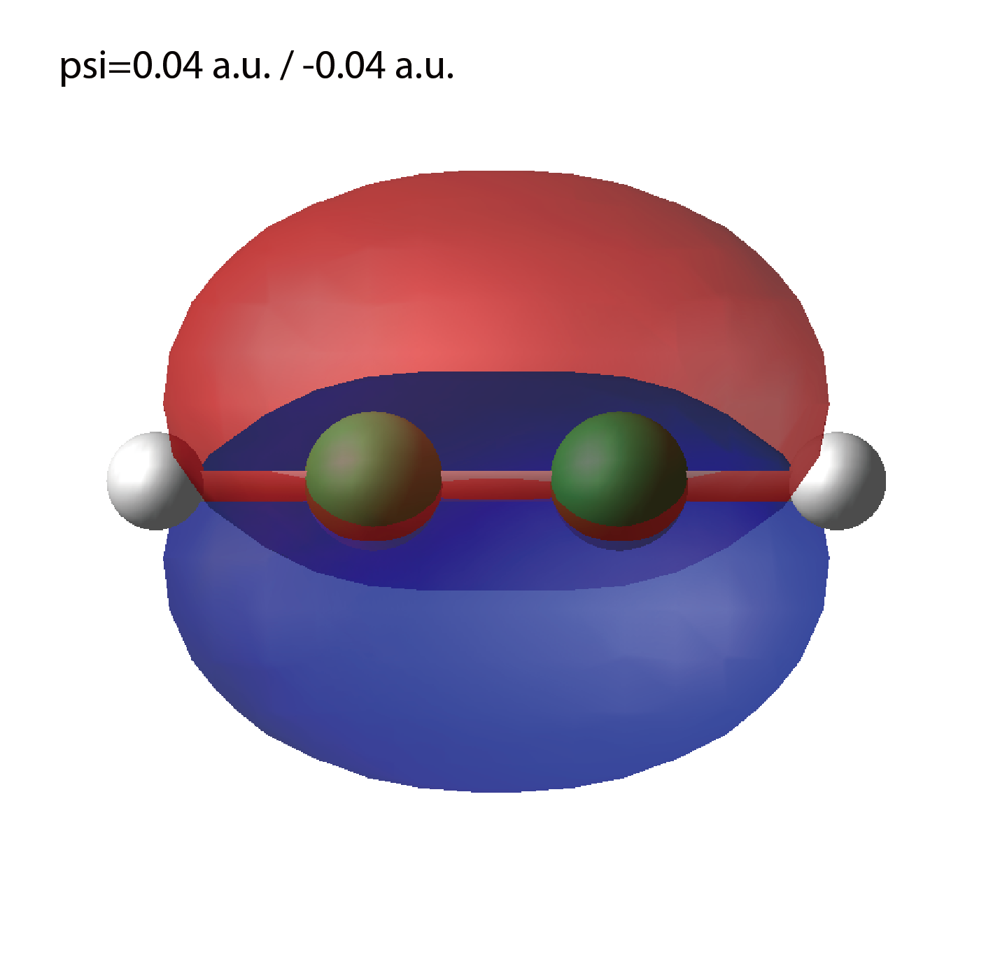
Highest occupied molecular orbital (HOMO)
The output files psi_ob1.cube, psi_ob2.cube, ... are used to create the image.
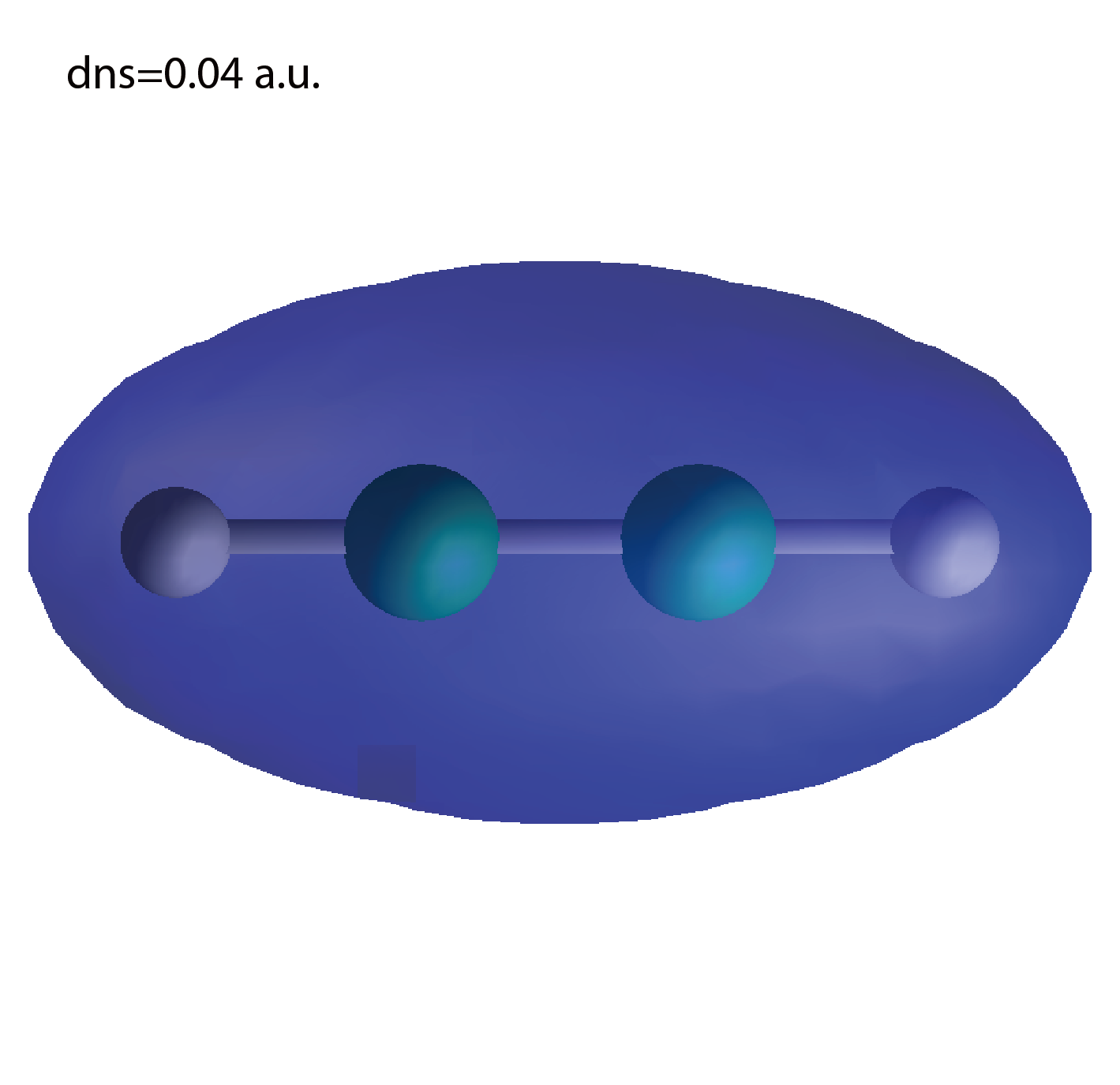
Electron density
The output files dns.cube, ... are used to create the image.
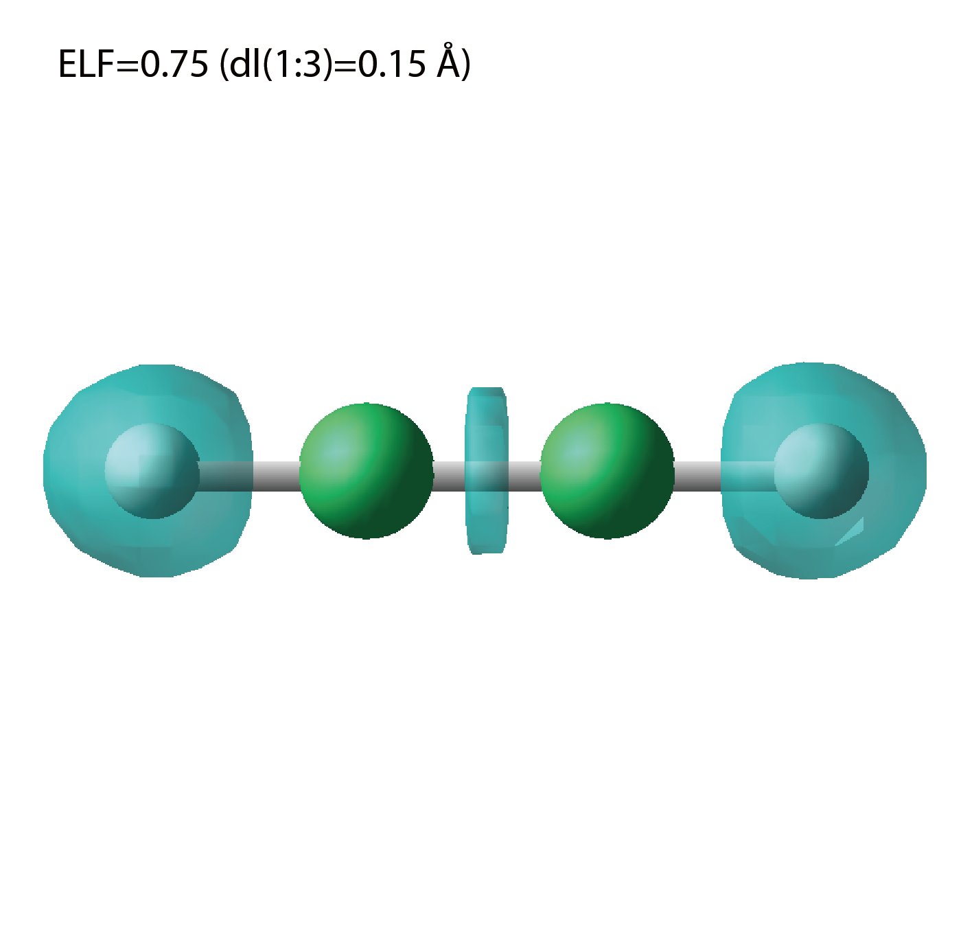
Electron localization function
The output files elf.cube, ... are used to create the image.
Exercise-2: Polarizability and photoabsorption of C2H2 molecule
In this exercise, we learn the linear response calculation in the acetylene (C2H2) molecule, solving the time-dependent Kohn-Sham equation. The linear response calculation provides the polarizability and the oscillator strength distribution of the molecule. This exercise should be carried out after finishing the ground state calculation that was explained in Exercise-1. In the calculation, an impulsive perturbation is applied to all electrons in the C2H2 molecule along the molecular axis which we take z axis. Then a time evolution calculation is carried out without any external fields. During the calculation, the electric dipole moment is monitored. After the time evolution calculation, a time-frequency Fourier transformation is carried out for the electric dipole moment to obtain the frequency-dependent polarizability. The imaginary part of the frequency-dependent polarizability is proportional to the oscillator strength distribution and the photoabsorption cross section.
Input files
To run the code, the input file C2H2_rt_response.inp that contains input keywords and their values for the linear response calculation is required. The directory restart that is created in the ground state calculation as data_for_restart and pseudopotential files are also required. The pseudopotential files should be the same as those used in the ground state calculation. The input files are in samples.
| name | description |
| C2H2_rt_response.inp | input file that contains input keywords and their values |
| C_rps.dat | pseodupotential file for carbon |
| H_rps.dat | pseudopotential file for hydrogen |
| restart | directory created in the ground state calculation (rename the directory from data_for_restart to restart) |
In the input file C2H2_rt_response.inp, input keywords are specified. Most of them are mandatory to execute the linear response calculation. This will help you to prepare the input file for other systems that you want to calculate. A complete list of the input keywords that can be used in the input file can be found in List of all input keywords.
!########################################################################################!
! Excercise 02: Polarizability and photoabsorption of C2H2 molecule                      !
!----------------------------------------------------------------------------------------!
! * The detail of this excercise is expained in our manual(see chapter: 'Exercises').    !
!   The manual can be obtained from: https://salmon-tddft.jp/documents.html              !
! * Input format consists of group of keywords like:                                     !
!     &group                                                                             !
!       input keyword = xxx                                                              !
!     /                                                                                  !
!   (see chapter: 'List of all input keywords' in the manual)                            !
!----------------------------------------------------------------------------------------!
! * Copy the ground state data directory('data_for_restart') (or make symbolic link)     !
!   calculated in 'samples/exercise_01_C2H2_gs/' and rename the directory to 'restart/'  !
!   in the current directory.                                                            !
!########################################################################################!

&calculation
  !type of theory
  theory = 'tddft_response'
/

&control
  !common name of output files
  sysname = 'C2H2'
/

&units
  !units used in input and output files
  unit_system = 'A_eV_fs'
/

&system
  !periodic boundary condition
  yn_periodic = 'n'

  !grid box size(x,y,z)
  al(1:3) = 16.0d0, 16.0d0, 16.0d0

  !number of elements, atoms, electrons and states(orbitals)
  nelem  = 2
  natom  = 4
  nelec  = 10
  nstate = 6
/

&pseudo
  !name of input pseudo potential file
  file_pseudo(1) = './C_rps.dat'
  file_pseudo(2) = './H_rps.dat'

  !atomic number of element
  izatom(1) = 6
  izatom(2) = 1

  !angular momentum of pseudopotential that will be treated as local
  lloc_ps(1) = 1
  lloc_ps(2) = 0
  !--- Caution ---------------------------------------!
  ! Indices must correspond to those in &atomic_coor. !
  !---------------------------------------------------!
/

&functional
  !functional('PZ' is Perdew-Zunger LDA: Phys. Rev. B 23, 5048 (1981).)
  xc = 'PZ'
/

&rgrid
  !spatial grid spacing(x,y,z)
  dl(1:3) = 0.25d0, 0.25d0, 0.25d0
/

&tgrid
  !time step size and number of time grids(steps)
  dt = 1.25d-3
  nt = 5000
/

&emfield
  !envelope shape of the incident pulse('impulse': impulsive field)
  ae_shape1 = 'impulse'

  !polarization unit vector(real part) for the incident pulse(x,y,z)
  epdir_re1(1:3) = 0.0d0, 0.0d0, 1.0d0
  !--- Caution ---------------------------------------------------------!
  ! Defenition of the incident pulse is wrriten in:                     !
  ! https://www.sciencedirect.com/science/article/pii/S0010465518303412 !
  !---------------------------------------------------------------------!
/

&analysis
  !energy grid size and number of energy grids for output files
  de      = 1.0d-2
  nenergy = 3000
/

&atomic_coor
  !cartesian atomic coodinates
  'C'    0.000000    0.000000    0.599672  1
  'H'    0.000000    0.000000    1.662257  2
  'C'    0.000000    0.000000   -0.599672  1
  'H'    0.000000    0.000000   -1.662257  2
  !--- Format ---------------------------------------------------!
  ! 'symbol' x y z index(correspond to that of pseudo potential) !
  !--------------------------------------------------------------!
/
We present their explanations below:
Required and recommended variables
&calculation
Mandatory: theory
&calculation
  !type of theory
  theory = 'tddft_response'
/
This indicates that the real time (RT) calculation to obtain response function is carried out in the present job. See &calculation in Inputs for detail.
&control
Mandatory: none
&control
  !common name of output files
  sysname = 'C2H2'
/
'C2H2' defined by sysname = 'C2H2' will be used in the filenames of
output files.
&units
Mandatory: none
&units
  !units used in input and output files
  unit_system = 'A_eV_fs'
/
This input keyword specifies the unit system to be used in the input file. If you do not specify it, atomic unit will be used. See &units in Inputs for detail.
&system
Mandatory: iperiodic, al, nelem, natom, nelec, nstate
&system
  !periodic boundary condition
  yn_periodic = 'n'

  !grid box size(x,y,z)
  al(1:3) = 16.0d0, 16.0d0, 16.0d0

  !number of elements, atoms, electrons and states(orbitals)
  nelem  = 2
  natom  = 4
  nelec  = 10
  nstate = 6
/
These input keywords and their values should be the same as those used in the ground state calculation. See &system in Exercise-1.
&pseudo
Mandatory: file_pseudo, izatom
&pseudo
  !name of input pseudo potential file
  file_pseudo(1) = './C_rps.dat'
  file_pseudo(2) = './H_rps.dat'

  !atomic number of element
  izatom(1) = 6
  izatom(2) = 1

  !angular momentum of pseudopotential that will be treated as local
  lloc_ps(1) = 1
  lloc_ps(2) = 0
  !--- Caution ---------------------------------------!
  ! Indices must correspond to those in &atomic_coor. !
  !---------------------------------------------------!
/
These input keywords and their values should be the same as those used in the ground state calculation. See &pseudo in Exercise-1.
&functional
Mandatory: xc
&functional
  !functional('PZ' is Perdew-Zunger LDA: Phys. Rev. B 23, 5048 (1981).)
  xc = 'PZ'
/
This indicates that the local density approximation with the Perdew-Zunger functional is used.
&rgrid
Mandatory: dl or num_rgrid
&rgrid
  !spatial grid spacing(x,y,z)
  dl(1:3) = 0.25d0, 0.25d0, 0.25d0
/
dl(1:3) = 0.25d0, 0.25d0, 0.25d0 specifies the grid spacings
in three Cartesian directions. This must be the same as
that in the ground state calculation.
See &rgrid in Inputs for more information.
&tgrid
Mandatory: dt, nt
&tgrid
  !time step size and number of time grids(steps)
  dt = 1.25d-3
  nt = 5000
/
dt=1.25d-3 specifies the time step of the time evolution
calculation. nt=5000 specifies the number of time steps in the
calculation.
&emfield
Mandatory: ae_shape1
&emfield
  !envelope shape of the incident pulse('impulse': impulsive field)
  ae_shape1 = 'impulse'

  !polarization unit vector(real part) for the incident pulse(x,y,z)
  epdir_re1(1:3) = 0.0d0, 0.0d0, 1.0d0
  !--- Caution ---------------------------------------------------------!
  ! Defenition of the incident pulse is wrriten in:                     !
  ! https://www.sciencedirect.com/science/article/pii/S0010465518303412 !
  !---------------------------------------------------------------------!
/
ae_shape1 = 'impulse' indicates that a weak impulse is applied to
all electrons at t=0. epdir_re1(1:3) = 0.0d0, 0.0d0, 1.0d0 specify a unit vector that
indicates the direction of the impulse.
See &emfield in Inputs for details.
&atomic_coor
Mandatory: atomic_coor or atomic_red_coor (it may be provided as a separate file)
&atomic_coor
  !cartesian atomic coodinates
  'C'    0.000000    0.000000    0.599672  1
  'H'    0.000000    0.000000    1.662257  2
  'C'    0.000000    0.000000   -0.599672  1
  'H'    0.000000    0.000000   -1.662257  2
  !--- Format ---------------------------------------------------!
  ! 'symbol' x y z index(correspond to that of pseudo potential) !
  !--------------------------------------------------------------!
/
Cartesian coordinates of atoms. The first column indicates the element. Next three columns specify Cartesian coordinates of the atoms. The number in the last column labels the element. They must be the same as those in the ground state calculation.
Output files
After the calculation, following output files are created in the directory that you run the code,
| file name | description |
| C2H2_response.data | polarizability and oscillator strength distribution as functions of energy |
| C2H2_rt.data | components of change of dipole moment (electrons/plus definition) and total dipole moment (electrons/minus + ions/plus) as functions of time |
| C2H2_rt_energy.data | components of total energy and difference of total energy as functions of time |
| PS_C_KY_n.dat | information on pseodupotential file for carbon atom |
| PS_H_KY_n.dat | information on pseodupotential file for hydrogen atom |
Explanations of the output files are below:
C2H2_response.data
Time-frequency Fourier transformation of the dipole moment gives the polarizability of the system. Then the strength function is calculated.
# Fourier-transform spectra:
# alpha: Polarizability
# df/dE: Strength function
# 1:Energy[eV] 2:Re(alpha_x)[Augstrom^2/V] 3:Re(alpha_y)[Augstrom^2/V] 4:Re(alpha_z)[Augstrom^2/V] 5:Im(alpha_x)[Augstrom^2/V] 6:Im(alpha_y)[Augstrom^2/V] 7:Im(alpha_z)[Augstrom^2/V] 8:df_x/dE[none] 9:df_y/dE[none] 10:df_z/dE[none]
C2H2_rt.data
Results of time evolution calculation for vector potential, electric field, and dipole moment.
# Real time calculation:
# Ac_ext: External vector potential field
# E_ext: External electric field
# Ac_tot: Total vector potential field
# E_tot: Total electric field
# ddm_e: Change of dipole moment (electrons/plus definition)
# dm: Total dipole moment (electrons/minus + ions/plus)
# 1:Time[fs] 2:Ac_ext_x[fs*V/Angstrom] 3:Ac_ext_y[fs*V/Angstrom] 4:Ac_ext_z[fs*V/Angstrom] 5:E_ext_x[V/Angstrom] 6:E_ext_y[V/Angstrom] 7:E_ext_z[V/Angstrom] 8:Ac_tot_x[fs*V/Angstrom] 9:Ac_tot_y[fs*V/Angstrom] 10:Ac_tot_z[fs*V/Angstrom] 11:E_tot_x[V/Angstrom] 12:E_tot_y[V/Angstrom] 13:E_tot_z[V/Angstrom] 14:ddm_e_x[Angstrom] 15:ddm_e_y[Angstrom] 16:ddm_e_z[Angstrom] 17:dm_x[Angstrom] 18:dm_y[Angstrom] 19:dm_z[Angstrom]
C2H2_rt_energy.data
Eall and Eall-Eall0 are total energy and electronic excitation energy, respectively.
# Real time calculation:
# Eall: Total energy
# Eall0: Initial energy
# 1:Time[fs] 2:Eall[eV] 3:Eall-Eall0[eV]
Exercise-3: Electron dynamics in C2H2 molecule under a pulsed electric field
In this exercise, we learn the calculation of the electron dynamics in the acetylene (C2H2) molecule under a pulsed electric field, solving the time-dependent Kohn-Sham equation. As outputs of the calculation, such quantities as the total energy and the electric dipole moment of the system as functions of time are calculated. This tutorial should be carried out after finishing the ground state calculation that was explained in Exercise-1. In the calculation, a pulsed electric field that has cos^2 envelope shape is applied. The parameters that characterize the pulsed field such as magnitude, frequency, polarization direction, and carrier envelope phase are specified in the input file.
Input files
To run the code, following files in samples are used. The directory restart is created in the ground state calculation as data_for_restart. Pseudopotential files are already used in the ground state calculation. Therefore, C2H2_rt_pulse.inp that specifies input keywords and their values for the pulsed electric field calculation is the only file that the users need to prepare.
| file name | description |
| C2H2_rt_pulse.inp | input file that contain input keywords and their values. |
| C_rps.dat | pseodupotential file for carbon |
| H_rps.dat | pseudopotential file for hydrogen |
| restart | directory created in the ground state calculation (rename the directory from data_for_restart to restart) |
In the input file C2H2_rt_pulse.inp, input keywords are specified. Most of them are mandatory to execute the calculation of electron dynamics induced by a pulsed electric field. This will help you to prepare the input file for other systems and other pulsed electric fields that you want to calculate. A complete list of the input keywords that can be used in the input file can be found in List of all input keywords.
!########################################################################################!
! Excercise 03:  Electron dynamics in C2H2 molecule under a pulsed electric field        !
!----------------------------------------------------------------------------------------!
! * The detail of this excercise is expained in our manual(see chapter: 'Exercises').    !
!   The manual can be obtained from: https://salmon-tddft.jp/documents.html              !
! * Input format consists of group of keywords like:                                     !
!     &group                                                                             !
!       input keyword = xxx                                                              !
!     /                                                                                  !
!   (see chapter: 'List of all input keywords' in the manual)                            !
!----------------------------------------------------------------------------------------!
! * Copy the ground state data directory('data_for_restart') (or make symbolic link)     !
!   calculated in 'samples/exercise_01_C2H2_gs/' and rename the directory to 'restart/'  !
!   in the current directory.                                                            !
!########################################################################################!

&calculation
  !type of theory
  theory = 'tddft_pulse'
/

&control
  !common name of output files
  sysname = 'C2H2'
/

&units
  !units used in input and output files
  unit_system = 'A_eV_fs'
/

&system
  !periodic boundary condition
  yn_periodic = 'n'

  !grid box size(x,y,z)
  al(1:3) = 16.0d0, 16.0d0, 16.0d0

  !number of elements, atoms, electrons and states(orbitals)
  nelem  = 2
  natom  = 4
  nelec  = 10
  nstate = 6
/

&pseudo
  !name of input pseudo potential file
  file_pseudo(1) = './C_rps.dat'
  file_pseudo(2) = './H_rps.dat'

  !atomic number of element
  izatom(1) = 6
  izatom(2) = 1

  !angular momentum of pseudopotential that will be treated as local
  lloc_ps(1) = 1
  lloc_ps(2) = 0
  !--- Caution ---------------------------------------!
  ! Indices must correspond to those in &atomic_coor. !
  !---------------------------------------------------!
/

&functional
  !functional('PZ' is Perdew-Zunger LDA: Phys. Rev. B 23, 5048 (1981).)
  xc = 'PZ'
/

&rgrid
  !spatial grid spacing(x,y,z)
  dl(1:3) = 0.25d0, 0.25d0, 0.25d0
/

&tgrid
  !time step size and number of time grids(steps)
  dt = 1.25d-3
  nt = 5000
/

&emfield
  !envelope shape of the incident pulse('Ecos2': cos^2 type envelope for scalar potential)
  ae_shape1 = 'Ecos2'

  !peak intensity(W/cm^2) of the incident pulse
  I_wcm2_1 = 1.00d8

  !duration of the incident pulse
  tw1 = 6.00d0

  !mean photon energy(average frequency multiplied by the Planck constant) of the incident pulse
  omega1 = 9.28d0

  !polarization unit vector(real part) for the incident pulse(x,y,z)
  epdir_re1(1:3) = 0.00d0, 0.00d0, 1.00d0

  !carrier emvelope phase of the incident pulse
  !(phi_cep1 must be 0.25 + 0.5 * n(integer) when ae_shape1 = 'Ecos2')
  phi_cep1 = 0.75d0
  !--- Caution ---------------------------------------------------------!
  ! Defenition of the incident pulse is wrriten in:                     !
  ! https://www.sciencedirect.com/science/article/pii/S0010465518303412 !
  !---------------------------------------------------------------------!
/

&atomic_coor
  !cartesian atomic coodinates
  'C'    0.000000    0.000000    0.599672  1
  'H'    0.000000    0.000000    1.662257  2
  'C'    0.000000    0.000000   -0.599672  1
  'H'    0.000000    0.000000   -1.662257  2
  !--- Format ---------------------------------------------------!
  ! 'symbol' x y z index(correspond to that of pseudo potential) !
  !--------------------------------------------------------------!
/
We present explanations of the input keywords that appear in the input file below:
Required and recommened variables
&calculation
Mandatory: theory
&calculation
  !type of theory
  theory = 'tddft_pulse'
/
This indicates that the real time (RT) calculation for a pulse response is carried out in the present job. See &calculation in Inputs for detail.
&control
Mandatory: none
&control
  !common name of output files
  sysname = 'C2H2'
/
'C2H2' defined by sysname = 'C2H2' will be used
in the filenames of output files.
&units
Mandatory: none
&units
  !units used in input and output files
  unit_system = 'A_eV_fs'
/
This input keyword specifies the unit system to be used in the input file. If you do not specify it, atomic unit will be used. See &units in Inputs for detail.
&system
Mandatory: yn_periodic, al, nelem, natom, nelectron, nstate
&system
  !periodic boundary condition
  yn_periodic = 'n'

  !grid box size(x,y,z)
  al(1:3) = 16.0d0, 16.0d0, 16.0d0

  !number of elements, atoms, electrons and states(orbitals)
  nelem  = 2
  natom  = 4
  nelec  = 10
  nstate = 6
/
These input keywords and their values should be the same as those used in the ground state calculation. See &system in Exercise-1.
&pseudo
Mandatory: file_pseudo, izatom
&pseudo
  !name of input pseudo potential file
  file_pseudo(1) = './C_rps.dat'
  file_pseudo(2) = './H_rps.dat'

  !atomic number of element
  izatom(1) = 6
  izatom(2) = 1

  !angular momentum of pseudopotential that will be treated as local
  lloc_ps(1) = 1
  lloc_ps(2) = 0
  !--- Caution ---------------------------------------!
  ! Indices must correspond to those in &atomic_coor. !
  !---------------------------------------------------!
/
These input keywords and their values should be the same as those used in the ground state calculation. See &pseudo in Exercise-1.
&functional
Mandatory: xc
&functional
  !functional('PZ' is Perdew-Zunger LDA: Phys. Rev. B 23, 5048 (1981).)
  xc = 'PZ'
/
This indicates that the local density approximation with the Perdew-Zunger functional is used.
&rgrid
Mandatory: dl or num_rgrid
&rgrid
  !spatial grid spacing(x,y,z)
  dl(1:3) = 0.25d0, 0.25d0, 0.25d0
/
dl(1:3) = 0.25d0, 0.25d0, 0.25d0 specifies the grid spacings
in three Cartesian directions. This must be the same as
that in the ground state calculation.
See &rgrid in Inputs for more information.
&tgrid
Mandatory: dt, nt
&tgrid
  !time step size and number of time grids(steps)
  dt = 1.25d-3
  nt = 5000
/
dt = 1.25d-3 specifies the time step of the time evolution
calculation. nt = 5000 specifies the number of time steps in the
calculation.
&emfield
Mandatory: ae_shape1, {I_wcm2_1 or E_amplitude1}, tw1, omega1, epdir_re1, phi_cep1
&emfield
  !envelope shape of the incident pulse('Ecos2': cos^2 type envelope for scalar potential)
  ae_shape1 = 'Ecos2'

  !peak intensity(W/cm^2) of the incident pulse
  I_wcm2_1 = 1.00d8

  !duration of the incident pulse
  tw1 = 6.00d0

  !mean photon energy(average frequency multiplied by the Planck constant) of the incident pulse
  omega1 = 9.28d0

  !polarization unit vector(real part) for the incident pulse(x,y,z)
  epdir_re1(1:3) = 0.00d0, 0.00d0, 1.00d0

  !carrier emvelope phase of the incident pulse
  !(phi_cep1 must be 0.25 + 0.5 * n(integer) when ae_shape1 = 'Ecos2')
  phi_cep1 = 0.75d0
  !--- Caution ---------------------------------------------------------!
  ! Defenition of the incident pulse is wrriten in:                     !
  ! https://www.sciencedirect.com/science/article/pii/S0010465518303412 !
  !---------------------------------------------------------------------!
/
These input keywords specify the pulsed electric field applied to the system.
ae_shape1 = 'Ecos2' indicates that the envelope of the pulsed
electric field has a cos^2 shape.
I_wcm2_1 = 1.00d8 specifies the maximum intensity of the
applied electric field in unit of W/cm^2.
tw1 = 6.00d0 specifies the pulse duration. Note that it is not the
FWHM but a full duration of the cos^2 envelope.
omega1 = 9.28d0 specifies the average photon energy (frequency
multiplied with hbar).
epdir_re1(1:3) = 0.00d0, 0.00d0, 1.00d0 specifies the real part of the unit
polarization vector of the pulsed electric field. Using the real
polarization vector, it describes a linearly polarized pulse.
phi_cep1 = 0.75d0 specifies the carrier envelope phase of the pulse.
As noted above, 'phi_cep1' must be 0.75 (or 0.25) if one employs 'Ecos2'
pulse shape, since otherwise the time integral of the electric field
does not vanish.
See &emfield in Inputs for details.
&atomic_coor
Mandatory: atomic_coor or atomic_red_coor (it may be provided as a separate file)
&atomic_coor
  !cartesian atomic coodinates
  'C'    0.000000    0.000000    0.599672  1
  'H'    0.000000    0.000000    1.662257  2
  'C'    0.000000    0.000000   -0.599672  1
  'H'    0.000000    0.000000   -1.662257  2
  !--- Format ---------------------------------------------------!
  ! 'symbol' x y z index(correspond to that of pseudo potential) !
  !--------------------------------------------------------------!
/
Cartesian coordinates of atoms. The first column indicates the element. Next three columns specify Cartesian coordinates of the atoms. The number in the last column labels the element. They must be the same as those in the ground state calculation.
Output files
After the calculation, following output files are created in the directory that you run the code,
| file name | description |
| C2H2_pulse.data | dipole moment as functions of energy |
| C2H2_rt.data | components of change of dipole moment (electrons/plus definition) and total dipole moment (electrons/minus + ions/plus) as functions of time |
| C2H2_rt_energy.data | components of total energy and difference of total energy as functions of time |
| PS_C_KY_n.dat | information on pseodupotential file for carbon atom |
| PS_H_KY_n.dat | information on pseodupotential file for hydrogen atom |
Explanations of the files are described below:
C2H2_pulse.data
Time-frequency Fourier transformation of the dipole moment.
# Fourier-transform spectra:
# energy: Frequency
# dm: Dopile moment
# 1:energy[eV] 2:Re(dm_x)[fs*Angstrom] 3:Re(dm_y)[fs*Angstrom] 4:Re(dm_z)[fs*Angstrom] 5:Im(dm_x)[fs*Angstrom] 6:Im(dm_y)[fs*Angstrom] 7:Im(dm_z)[fs*Angstrom] 8:|dm_x|^2[fs^2*Angstrom^2] 9:|dm_y|^2[fs^2*Angstrom^2] 10:|dm_z|^2[fs^2*Angstrom^2]
C2H2_rt.data
Results of time evolution calculation for vector potential, electric field, and dipole moment.
# Real time calculation:
# Ac_ext: External vector potential field
# E_ext: External electric field
# Ac_tot: Total vector potential field
# E_tot: Total electric field
# ddm_e: Change of dipole moment (electrons/plus definition)
# dm: Total dipole moment (electrons/minus + ions/plus)
# 1:Time[fs] 2:Ac_ext_x[fs*V/Angstrom] 3:Ac_ext_y[fs*V/Angstrom] 4:Ac_ext_z[fs*V/Angstrom] 5:E_ext_x[V/Angstrom] 6:E_ext_y[V/Angstrom] 7:E_ext_z[V/Angstrom] 8:Ac_tot_x[fs*V/Angstrom] 9:Ac_tot_y[fs*V/Angstrom] 10:Ac_tot_z[fs*V/Angstrom] 11:E_tot_x[V/Angstrom] 12:E_tot_y[V/Angstrom] 13:E_tot_z[V/Angstrom] 14:ddm_e_x[Angstrom] 15:ddm_e_y[Angstrom] 16:ddm_e_z[Angstrom] 17:dm_x[Angstrom] 18:dm_y[Angstrom] 19:dm_z[Angstrom]
C2H2_rt_energy.data
Eall and Eall-Eall0 are total energy and electronic excitation energy, respectively.
# Real time calculation:
# Eall: Total energy
# Eall0: Initial energy
# 1:Time[fs] 2:Eall[eV] 3:Eall-Eall0[eV]
Crystalline silicon (periodic solids)
Exercise-4: Ground state of crystalline silicon
In this exercise, we learn the the ground state calculation of the crystalline silicon of a diamond structure. Calculation is done in a cubic unit cell that contains eight silicon atoms. This exercise will be useful to learn how to set up calculations in SALMON for any periodic systems such as crystalline solid.
Input files
To run the code, following files in samples are used:
| file name | description |
| Si_gs.inp | input file that contains input keywords and their values |
| Si_rps.dat | pseodupotential file for silicon atom |
In the input file Si_gs.inp, input keywords are specified. Most of them are mandatory to execute the ground state calculation. This will help you to prepare an input file for other systems that you want to calculate. A complete list of the input keywords that can be used in the input file can be found in List of all input keywords.
!########################################################################################!
! Excercise 04: Ground state of crystalline silicon(periodic solids)                     !
!----------------------------------------------------------------------------------------!
! * The detail of this excercise is expained in our manual(see chapter: 'Exercises').    !
!   The manual can be obtained from: https://salmon-tddft.jp/documents.html              !
! * Input format consists of group of keywords like:                                     !
!     &group                                                                             !
!       input keyword = xxx                                                              !
!     /                                                                                  !
!   (see chapter: 'List of all input keywords' in the manual)                            !
!########################################################################################!

&calculation
  !type of theory
  theory = 'dft'
/

&control
  !common name of output files
  sysname = 'Si'
/

&units
  !units used in input and output files
  unit_system = 'a.u.'
/

&system
  !periodic boundary condition
  yn_periodic = 'y'

  !grid box size(x,y,z)
  al(1:3) = 10.26d0, 10.26d0, 10.26d0

  !number of elements, atoms, electrons and states(bands)
  nelem  = 1
  natom  = 8
  nelec  = 32
  nstate = 32
/

&pseudo
  !name of input pseudo potential file
  file_pseudo(1) = './Si_rps.dat'

  !atomic number of element
  izatom(1) = 14

  !angular momentum of pseudopotential that will be treated as local
  lloc_ps(1) = 2
  !--- Caution -------------------------------------------!
  ! Index must correspond to those in &atomic_red_coor.   !
  !-------------------------------------------------------!
/

&functional
  !functional('PZ' is Perdew-Zunger LDA: Phys. Rev. B 23, 5048 (1981).)
  xc = 'PZ'
/

&rgrid
  !number of spatial grids(x,y,z)
  num_rgrid(1:3) = 12, 12, 12
/

&kgrid
  !number of k-points(x,y,z)
  num_kgrid(1:3) = 4, 4, 4
/

&scf
  !maximum number of scf iteration and threshold of convergence
  nscf      = 300
  threshold = 1.0d-9
/

&atomic_red_coor
  !cartesian atomic reduced coodinates
  'Si'       .0      .0      .0      1
  'Si'       .25     .25     .25     1
  'Si'       .5      .0      .5      1
  'Si'       .0      .5      .5      1
  'Si'       .5      .5      .0      1
  'Si'       .75     .25     .75     1
  'Si'       .25     .75     .75     1
  'Si'       .75     .75     .25     1
  !--- Format ---------------------------------------------------!
  ! 'symbol' x y z index(correspond to that of pseudo potential) !
  !--------------------------------------------------------------!
/
We present their explanations below:
Required and recommened variables
&calculation
Mandatory: theory
&calculation
  !type of theory
  theory = 'dft'
/
This indicates that the ground state calculation by DFT is carried out in the present job. See &calculation in Inputs for detail.
&control
Mandatory: none
&control
  !common name of output files
  sysname = 'Si'
/
'Si' defined by sysname = 'Si' will be used in the filenames of
output files.
&units
Mandatory: none
&units
  !units used in input and output files
  unit_system = 'a.u.'
/
This input keyword specifies the unit system to be used in the input and output files. If you do not specify it, atomic unit will be used. See &units in Inputs for detail.
&system
Mandatory: yn_periodic, al, nelem, natom, nelec, nstate
&system
  !periodic boundary condition
  yn_periodic = 'y'

  !grid box size(x,y,z)
  al(1:3) = 10.26d0, 10.26d0, 10.26d0

  !number of elements, atoms, electrons and states(bands)
  nelem  = 1
  natom  = 8
  nelec  = 32
  nstate = 32
/
yn_periodic = 'y' indicates that three dimensional periodic boundary condition (bulk crystal) is assumed.
al(1:3) = 10.26d0, 10.26d0, 10.26d0 specifies the lattice constans of the unit cell.
nelem = 1 and natom = 8 indicate the number of elements and the number of atoms in the system, respectively.
nelec = 32 indicate the number of valence electrons in the system.
nstate = 32 indicates the number of Kohn-Sham orbitals to be solved.
See &system in Inputs for more information.
&pseudo
Mandatory: file_pseudo, izatom
&pseudo
  !name of input pseudo potential file
  file_pseudo(1) = './Si_rps.dat'

  !atomic number of element
  izatom(1) = 14

  !angular momentum of pseudopotential that will be treated as local
  lloc_ps(1) = 2
  !--- Caution -------------------------------------------!
  ! Index must correspond to those in &atomic_red_coor.   !
  !-------------------------------------------------------!
/
file_pseudo(1) = './Si_rps.dat' indicates the pseudopotential filename of element.
izatom(1) = 14 indicates the atomic number of the element.
lloc_ps(1) = 2 indicate the angular momentum of the pseudopotential that will be treated as local.
&functional
Mandatory: xc
&functional
  !functional('PZ' is Perdew-Zunger LDA: Phys. Rev. B 23, 5048 (1981).)
  xc = 'PZ'
/
This indicates that the local density approximation with the Perdew-Zunger functional is used.
&rgrid
Mandatory: dl or num_rgrid
&rgrid
  !number of spatial grids(x,y,z)
  num_rgrid(1:3) = 12, 12, 12
/
num_rgrid(1:3) = 12, 12, 12 specifies the number of the grids for each Cartesian direction.
See &rgrid in Inputs for more information.
&rgrid
Mandatory: none
&kgrid
  !number of k-points(x,y,z)
  num_kgrid(1:3) = 4, 4, 4
/
This input keyword provides grid spacing of k-space for periodic systems.
&scf
Mandatory: nscf, threshold
&scf
  !maximum number of scf iteration and threshold of convergence
  nscf      = 300
  threshold = 1.0d-9
/
nscf is the number of scf iterations.
The scf loop in the ground state calculation ends before the number of
the scf iterations reaches nscf, if a convergence criterion is satisfied.
threshold = 1.0d-9 indicates threshold of the convergence for scf iterations.
&atomic_coor
Mandatory: atomic_coor or atomic_red_coor (it may be provided as a separate file)
&atomic_red_coor
  !cartesian atomic reduced coodinates
  'Si'       .0      .0      .0      1
  'Si'       .25     .25     .25     1
  'Si'       .5      .0      .5      1
  'Si'       .0      .5      .5      1
  'Si'       .5      .5      .0      1
  'Si'       .75     .25     .75     1
  'Si'       .25     .75     .75     1
  'Si'       .75     .75     .25     1
  !--- Format ---------------------------------------------------!
  ! 'symbol' x y z index(correspond to that of pseudo potential) !
  !--------------------------------------------------------------!
/
Cartesian coordinates of atoms are specified in a reduced coordinate system. First column indicates the element, next three columns specify reduced Cartesian coordinates of the atoms, and the last column labels the element.
Output files
After the calculation, following output files and a directory are created in the directory that you run the code,
| name | description |
| Si_info.data | information on ground state solution |
| Si_eigen.data | energy eigenvalues of orbitals |
| Si_k.data | k-point distribution |
| PS_Si_KY_n.dat | information on pseodupotential file for silicon atom |
| data_for_restart | directory where files used in the real-time calculation are contained |
Main results of the calculation such as orbital energies are included in Si_info.data. Explanations of the Si_info.data and other output files are below:
Si_info.data
Calculated orbital and total energies as well as parameters specified in the input file are shown in this file.
Si_eigen.data
1 particle energies.
#esp: single-particle energies (eigen energies)
#occ: occupation numbers, io: orbital index
# 1:io, 2:esp[a.u.], 3:occ
Si_k.data
k-point distribution.
# ik: k-point index
# kx,ky,kz: Reduced coordinate of k-points
# wk: Weight of k-point
# 1:ik[none] 2:kx[none] 3:ky[none] 4:kz[none] 5:wk[none]
# coefficients (2*pi/a [a.u.]) in kx, ky, kz
Exercise-5: Dielectric function of crystalline silicon
In this exercise, we learn the linear response calculation of the crystalline silicon of a diamond structure. Calculation is done in a cubic unit cell that contains eight silicon atoms. This exercise should be carried out after finishing the ground state calculation that was explained in Exercise-4. An impulsive perturbation is applied to all electrons in the unit cell along z direction. Since the dielectric function is isotropic in the diamond structure, calculated dielectric function should not depend on the direction of the perturbation. During the time evolution, electric current averaged over the unit cell volume is calculated. A time-frequency Fourier transformation of the electric current gives us a frequency-dependent conductivity. The dielectric function may be obtained from the conductivity using a standard relation.
Input files
To run the code, following files in samples are used:
In the input file Si_rt_response.inp, input keywords are specified. Most of them are mandatory to execute the calculation. This will help you to prepare the input file for other systems that you want to calculate. A complete list of the input keywords can be found in List of all input keywords.
!########################################################################################!
! Excercise 05: Dielectric function of crystalline silicon                               !
!----------------------------------------------------------------------------------------!
! * The detail of this excercise is expained in our manual(see chapter: 'Exercises').    !
!   The manual can be obtained from: https://salmon-tddft.jp/documents.html              !
! * Input format consists of group of keywords like:                                     !
!     &group                                                                             !
!       input keyword = xxx                                                              !
!     /                                                                                  !
!   (see chapter: 'List of all input keywords' in the manual)                            !
!----------------------------------------------------------------------------------------!
! * Copy the ground state data directory('data_for_restart') (or make symbolic link)     !
!   calculated in 'samples/exercise_04_bulkSi_gs/' and rename the directory to 'restart/'!
!   in the current directory.                                                            !
!########################################################################################!

&calculation
  !type of theory
  theory = 'tddft_response'
/

&control
  !common name of output files
  sysname = 'Si'
/

&units
  !units used in input and output files
  unit_system = 'a.u.'
/

&system
  !periodic boundary condition
  yn_periodic = 'y'

  !grid box size(x,y,z)
  al(1:3) = 10.26d0, 10.26d0, 10.26d0

  !number of elements, atoms, electrons and states(bands)
  nelem  = 1
  natom  = 8
  nelec  = 32
  nstate = 32
/

&pseudo
  !name of input pseudo potential file
  file_pseudo(1) = './Si_rps.dat'

  !atomic number of element
  izatom(1) = 14

  !angular momentum of pseudopotential that will be treated as local
  lloc_ps(1) = 2
  !--- Caution -------------------------------------------!
  ! Index must correspond to those in &atomic_red_coor.   !
  !-------------------------------------------------------!
/

&functional
  !functional('PZ' is Perdew-Zunger LDA: Phys. Rev. B 23, 5048 (1981).)
  xc = 'PZ'
/

&rgrid
  !number of spatial grids(x,y,z)
  num_rgrid(1:3) = 12, 12, 12
/

&kgrid
  !number of k-points(x,y,z)
  num_kgrid(1:3) = 4, 4, 4
/

&tgrid
  !time step size and number of time grids(steps)
  dt = 0.08d0
  nt = 6000
/

&emfield
  !envelope shape of the incident pulse('impulse': impulsive field)
  ae_shape1 = 'impulse'

  !polarization unit vector(real part) for the incident pulse(x,y,z)
  epdir_re1(1:3) = 0.00d0, 0.00d0, 1.00d0
  !--- Caution ---------------------------------------------------------!
  ! Defenition of the incident pulse is wrriten in:                     !
  ! https://www.sciencedirect.com/science/article/pii/S0010465518303412 !
  !---------------------------------------------------------------------!
/

&analysis
  !energy grid size and number of energy grids for output files
  de      = 1.0d-2
  nenergy = 5000
/

&atomic_red_coor
  !cartesian atomic reduced coodinates
  'Si'       .0      .0      .0      1
  'Si'       .25     .25     .25     1
  'Si'       .5      .0      .5      1
  'Si'       .0      .5      .5      1
  'Si'       .5      .5      .0      1
  'Si'       .75     .25     .75     1
  'Si'       .25     .75     .75     1
  'Si'       .75     .75     .25     1
  !--- Format ---------------------------------------------------!
  ! 'symbol' x y z index(correspond to that of pseudo potential) !
  !--------------------------------------------------------------!
/
We present explanations of the input keywords that appear in the input file below:
Required and recommened variables
&calculation
Mandatory: theory
&calculation
  !type of theory
  theory = 'tddft_response'
/
This indicates that the real time (RT) calculation to obtain response function is carried out in the present job. See &calculation in Inputs for detail.
&control
Mandatory: none
&control
  !common name of output files
  sysname = 'Si'
/
'Si' defined by sysname = 'Si' will be used in the filenames of output files.
&units
Mandatory: none
&units
  !units used in input and output files
  unit_system = 'a.u.'
/
This input keyword specifies the unit system to be used in the input and output files. If you do not specify it, atomic unit will be used. See &units in Inputs for detail.
&system
Mandatory: yn_periodic, al, state, nelem, nelem, natom, nelec, nstate
&system
  !periodic boundary condition
  yn_periodic = 'y'

  !grid box size(x,y,z)
  al(1:3) = 10.26d0, 10.26d0, 10.26d0

  !number of elements, atoms, electrons and states(bands)
  nelem  = 1
  natom  = 8
  nelec  = 32
  nstate = 32
/
These input keywords and their values should be the same as those used in the ground state calculation. See &system in Exercise-4.
&pseudo
Mandatory: file_pseudo, izatom
&pseudo
  !name of input pseudo potential file
  file_pseudo(1) = './Si_rps.dat'

  !atomic number of element
  izatom(1) = 14

  !angular momentum of pseudopotential that will be treated as local
  lloc_ps(1) = 2
  !--- Caution -------------------------------------------!
  ! Index must correspond to those in &atomic_red_coor.   !
  !-------------------------------------------------------!
/
These input keywords and their values should be the same as those used in the ground state calculation. See &pseudo in Exercise-4.
&functional
Mandatory: xc
&functional
  !functional('PZ' is Perdew-Zunger LDA: Phys. Rev. B 23, 5048 (1981).)
  xc = 'PZ'
/
This indicates that the local density approximation with the Perdew-Zunger functional is used.
&rgrid
Mandatory: dl or num_rgrid
&rgrid
  !number of spatial grids(x,y,z)
  num_rgrid(1:3) = 12, 12, 12
/
num_rgrid(1:3) = 12, 12, 12 specifies the number of the grids for each Cartesian direction.
This must be the same as that in the ground state calculation.
See &rgrid in Inputs for more information.
&kgrid
Mandatory: none
&kgrid
  !number of k-points(x,y,z)
  num_kgrid(1:3) = 4, 4, 4
/
This input keyword provides grid spacing of k-space for periodic systems. This must be the same as that in the ground state calculation.
&tgrid
Mandatory: dt, nt
&tgrid
  !time step size and number of time grids(steps)
  dt = 0.08d0
  nt = 6000
/
dt = 0.08d0 specifies the time step of the time evolution calculation.
nt = 6000 specifies the number of time steps in the calculation.
&emfield
Mandatory:ae_shape1
&emfield
  !envelope shape of the incident pulse('impulse': impulsive field)
  ae_shape1 = 'impulse'

  !polarization unit vector(real part) for the incident pulse(x,y,z)
  epdir_re1(1:3) = 0.00d0, 0.00d0, 1.00d0
  !--- Caution ---------------------------------------------------------!
  ! Defenition of the incident pulse is wrriten in:                     !
  ! https://www.sciencedirect.com/science/article/pii/S0010465518303412 !
  !---------------------------------------------------------------------!
/
as_shape1 = 'impulse' indicates that a weak impulsive field is applied to all electrons at t=0
epdir_re1(1:3) = 0.00d0, 0.00d0, 1.00d0 specify a unit vector that indicates the direction of the impulse.
See &emfield in Inputs for detail.
&analysis
Mandatory: none
&analysis
  !energy grid size and number of energy grids for output files
  de      = 1.0d-2
  nenergy = 5000
/
de = 1.0d-2 specifies the energy spacing in the time-frequency Fourier transformation.
nenergy = 5000 specifies the number of energy steps, and
&atomic_red_coor
Mandatory: atomic_coor or atomic_red_coor (they may be provided as a separate file)
&atomic_red_coor
  !cartesian atomic reduced coodinates
  'Si'       .0      .0      .0      1
  'Si'       .25     .25     .25     1
  'Si'       .5      .0      .5      1
  'Si'       .0      .5      .5      1
  'Si'       .5      .5      .0      1
  'Si'       .75     .25     .75     1
  'Si'       .25     .75     .75     1
  'Si'       .75     .75     .25     1
  !--- Format ---------------------------------------------------!
  ! 'symbol' x y z index(correspond to that of pseudo potential) !
  !--------------------------------------------------------------!
/
Cartesian coordinates of atoms are specified in a reduced coordinate system. First column indicates the element, next three columns specify reduced Cartesian coordinates of the atoms, and the last column labels the element.
Output files
After the calculation, following output files are created in the directory that you run the code,
| file name | description |
| Si_response.data | Fourier spectra of the conductivity and dielectric functions |
| Si_rt.data | vector potential, electric field, and matter current as functions of time |
| Si_rt_energy | components of total energy and difference of total energy as functions of time |
| PS_Si_KY_n.dat | information on pseodupotential file for silicon atom |
Explanations of the output files are described below:
Si_response.data
Time-frequency Fourier transformation of the macroscopic current gives the conductivity of the system. Then the dielectric function is calculated.
# Fourier-transform spectra:
# sigma: Conductivity
# eps: Dielectric constant
# 1:Energy[a.u.] 2:Re(sigma_x)[a.u.] 3:Re(sigma_y)[a.u.] 4:Re(sigma_z)[a.u.] 5:Im(sigma_x)[a.u.] 6:Im(sigma_y)[a.u.] 7:Im(sigma_z)[a.u.] 8:Re(eps_x)[none] 9:Re(eps_y)[none] 10:Re(eps_z)[none] 11:Im(eps_x)[none] 12:Im(eps_y)[none] 13:Im(eps_z)[none]
Si_rt.data
Results of time evolution calculation for vector potential, electric field, and matter current density.
# Real time calculation:
# Ac_ext: External vector potential field
# E_ext: External electric field
# Ac_tot: Total vector potential field
# E_tot: Total electric field
# Jm: Matter current density (electrons)
# 1:Time[a.u.] 2:Ac_ext_x[a.u.] 3:Ac_ext_y[a.u.] 4:Ac_ext_z[a.u.] 5:E_ext_x[a.u.] 6:E_ext_y[a.u.] 7:E_ext_z[a.u.] 8:Ac_tot_x[a.u.] 9:Ac_tot_y[a.u.] 10:Ac_tot_z[a.u.] 11:E_tot_x[a.u.] 12:E_tot_y[a.u.] 13:E_tot_z[a.u.]  14:Jm_x[a.u.] 15:Jm_y[a.u.] 16:Jm_z[a.u.]
Si_rt_energy
Eall and Eall-Eall0 are total energy and electronic excitation energy, respectively.
# Real time calculation:
# Eall: Total energy
# Eall0: Initial energy
# 1:Time[a.u.] 2:Eall[a.u.] 3:Eall-Eall0[a.u.]
Exercise-6: Electron dynamics in crystalline silicon under a pulsed electric field
In this exercise, we learn the calculation of electron dynamics in a unit cell of crystalline silicon of a diamond structure. Calculation is done in a cubic unit cell that contains eight silicon atoms. This exercise should be carried out after finishing the ground state calculation that was explained in Exercise-4. A pulsed electric field that has cos^2 envelope shape is applied. The parameters that characterize the pulsed field such as magnitude, frequency, polarization, and carrier envelope phase are specified in the input file.
Input files
To run the code, following files in samples are used:
| file name | description |
| Si_rt_pulse.inp | input file that contain input keywords and their values. |
| Si_rps.dat | pseodupotential file for Carbon |
| restart | directory created in the ground state calculation (rename the directory from data_for_restart to restart) |
In the input file Si_rt_pulse.inp, input keywords are specified. Most of them are mandatory to execute the calculation. This will help you to prepare the input file for other systems that you want to calculate. A complete list of the input keywords can be found in List of all input keywords.
!########################################################################################!
! Excercise 06: Electron dynamics in crystalline silicon under a pulsed electric field   !
!----------------------------------------------------------------------------------------!
! * The detail of this excercise is expained in our manual(see chapter: 'Exercises').    !
!   The manual can be obtained from: https://salmon-tddft.jp/documents.html              !
! * Input format consists of group of keywords like:                                     !
!     &group                                                                             !
!       input keyword = xxx                                                              !
!     /                                                                                  !
!   (see chapter: 'List of all input keywords' in the manual)                            !
!----------------------------------------------------------------------------------------!
! * Copy the ground state data directory('data_for_restart') (or make symbolic link)     !
!   calculated in 'samples/exercise_04_bulkSi_gs/' and rename the directory to 'restart/'!
!   in the current directory.                                                            !
!########################################################################################!

&calculation
  !type of theory
  theory = 'tddft_pulse'
/

&control
  !common name of output files
  sysname = 'Si'
/

&units
  !units used in input and output files
  unit_system = 'a.u.'
/

&system
  !periodic boundary condition
  yn_periodic = 'y'

  !grid box size(x,y,z)
  al(1:3) = 10.26d0, 10.26d0, 10.26d0

  !number of elements, atoms, electrons and states(bands)
  nelem  = 1
  natom  = 8
  nelec  = 32
  nstate = 32
/

&pseudo
  !name of input pseudo potential file
  file_pseudo(1) = './Si_rps.dat'

  !atomic number of element
  izatom(1) = 14

  !angular momentum of pseudopotential that will be treated as local
  lloc_ps(1) = 2
  !--- Caution -------------------------------------------!
  ! Index must correspond to those in &atomic_red_coor.   !
  !-------------------------------------------------------!
/

&functional
  !functional('PZ' is Perdew-Zunger LDA: Phys. Rev. B 23, 5048 (1981).)
  xc = 'PZ'
/

&rgrid
  !number of spatial grids(x,y,z)
  num_rgrid(1:3) = 12, 12, 12
/

&kgrid
  !number of k-points(x,y,z)
  num_kgrid(1:3) = 4, 4, 4
/

&tgrid
  !time step size and number of time grids(steps)
  dt = 0.08d0
  nt = 6000
/

&emfield
  !envelope shape of the incident pulse('Acos2': cos^2 type envelope for vector potential)
  ae_shape1 = 'Acos2'

  !peak intensity(W/cm^2) of the incident pulse
  I_wcm2_1 = 5.0d11

  !duration of the incident pulse
  tw1 = 441.195136248d0

  !mean photon energy(average frequency multiplied by the Planck constant) of the incident pulse
  omega1 = 0.05696145187d0

  !polarization unit vector(real part) for the incident pulse(x,y,z)
  epdir_re1(1:3) = 0.0d0, 0.0d0, 1.0d0
  !--- Caution ---------------------------------------------------------!
  ! Defenition of the incident pulse is wrriten in:                     !
  ! https://www.sciencedirect.com/science/article/pii/S0010465518303412 !
  !---------------------------------------------------------------------!
/

&atomic_red_coor
  !cartesian atomic reduced coodinates
  'Si'       .0      .0      .0      1
  'Si'       .25     .25     .25     1
  'Si'       .5      .0      .5      1
  'Si'       .0      .5      .5      1
  'Si'       .5      .5      .0      1
  'Si'       .75     .25     .75     1
  'Si'       .25     .75     .75     1
  'Si'       .75     .75     .25     1
  !--- Format ---------------------------------------------------!
  ! 'symbol' x y z index(correspond to that of pseudo potential) !
  !--------------------------------------------------------------!
/
We present explanations of the input keywords that appear in the input file below:
Required and recommened variables
&calculation
Mandatory: theory
&calculation
  !type of theory
  theory = 'tddft_response'
/
This indicates that the real time (RT) calculation to obtain response function is carried out in the present job. See &calculation in Inputs for detail.
&control
Mandatory: none
&control
  !common name of output files
  sysname = 'Si'
/
'Si' defined by sysname = 'Si' will be used in the filenames of output files.
&units
Mandatory: none
&units
  !units used in input and output files
  unit_system = 'a.u.'
/
This input keyword specifies the unit system to be used in the input and output files. If you do not specify it, atomic unit will be used. See &units in Inputs for detail.
&system
Mandatory: yn_periodic, al, state, nelem, nelem, natom, nelec, nstate
&system
  !periodic boundary condition
  yn_periodic = 'y'

  !grid box size(x,y,z)
  al(1:3) = 10.26d0, 10.26d0, 10.26d0

  !number of elements, atoms, electrons and states(bands)
  nelem  = 1
  natom  = 8
  nelec  = 32
  nstate = 32
/
These input keywords and their values should be the same as those used in the ground state calculation. See &system in Exercise-4.
&pseudo
Mandatory: file_pseudo, izatom
&pseudo
  !name of input pseudo potential file
  file_pseudo(1) = './Si_rps.dat'

  !atomic number of element
  izatom(1) = 14

  !angular momentum of pseudopotential that will be treated as local
  lloc_ps(1) = 2
  !--- Caution -------------------------------------------!
  ! Index must correspond to those in &atomic_red_coor.   !
  !-------------------------------------------------------!
/
These input keywords and their values should be the same as those used in the ground state calculation. See &pseudo in Exercise-4.
&functional
Mandatory: xc
&functional
  !functional('PZ' is Perdew-Zunger LDA: Phys. Rev. B 23, 5048 (1981).)
  xc = 'PZ'
/
This indicates that the local density approximation with the Perdew-Zunger functional is used.
&rgrid
Mandatory: dl or num_rgrid
&rgrid
  !number of spatial grids(x,y,z)
  num_rgrid(1:3) = 12, 12, 12
/
num_rgrid(1:3) = 12, 12, 12 specifies the number of the grids for each Cartesian direction.
This must be the same as that in the ground state calculation.
See &rgrid in Inputs for more information.
&kgrid
Mandatory: none
&kgrid
  !number of k-points(x,y,z)
  num_kgrid(1:3) = 4, 4, 4
/
This input keyword provides grid spacing of k-space for periodic systems. This must be the same as that in the ground state calculation.
&tgrid
Mandatory: dt, nt
&tgrid
  !time step size and number of time grids(steps)
  dt = 0.08d0
  nt = 6000
/
dt = 0.08d0 specifies the time step of the time evolution calculation.
nt = 6000 specifies the number of time steps in the calculation.
&emfield
Mandatory: ae_shape1, {I_wcm2_1 or E_amplitude1}, tw1, omega1, epdir_re1, phi_cep1
&emfield
  !envelope shape of the incident pulse('Acos2': cos^2 type envelope for vector potential)
  ae_shape1 = 'Acos2'

  !peak intensity(W/cm^2) of the incident pulse
  I_wcm2_1 = 5.0d11

  !duration of the incident pulse
  tw1 = 441.195136248d0

  !mean photon energy(average frequency multiplied by the Planck constant) of the incident pulse
  omega1 = 0.05696145187d0

  !polarization unit vector(real part) for the incident pulse(x,y,z)
  epdir_re1(1:3) = 0.0d0, 0.0d0, 1.0d0
  !--- Caution ---------------------------------------------------------!
  ! Defenition of the incident pulse is wrriten in:                     !
  ! https://www.sciencedirect.com/science/article/pii/S0010465518303412 !
  !---------------------------------------------------------------------!
/
These input keywords specify the pulsed electric field applied to the system.
ae_shape1 = 'Acos2' specifies the envelope of the pulsed electric
field, cos^2 envelope for the vector potential.
I_wcm2_1 = 5.0d11 specifies the maximum intensity of the
applied electric field in unit of W/cm^2.
tw1 = 441.195136248d0 specifies the pulse duration. Note that it
is not the FWHM but a full duration of the cos^2 envelope.
omega1 = 0.05696145187d0 specifies the average photon energy
(frequency multiplied with hbar).
epdir_re1(1:3) = 0.0d0, 0.0d0, 1.0d0 specify the real part of the unit polarization
vector of the pulsed electric field. Specifying only the real part, it
describes a linearly polarized pulse.
See &emfield in Inputs for detail.
&atomic_red_coor
Mandatory: atomic_coor or atomic_red_coor (they may be provided as a separate file)
&atomic_red_coor
  !cartesian atomic reduced coodinates
  'Si'       .0      .0      .0      1
  'Si'       .25     .25     .25     1
  'Si'       .5      .0      .5      1
  'Si'       .0      .5      .5      1
  'Si'       .5      .5      .0      1
  'Si'       .75     .25     .75     1
  'Si'       .25     .75     .75     1
  'Si'       .75     .75     .25     1
  !--- Format ---------------------------------------------------!
  ! 'symbol' x y z index(correspond to that of pseudo potential) !
  !--------------------------------------------------------------!
/
Cartesian coordinates of atoms are specified in a reduced coordinate system. First column indicates the element, next three columns specify reduced Cartesian coordinates of the atoms, and the last column labels the element.
Output files
After the calculation, following output files are created in the directory that you run the code,
| file name | description |
| Si_pulse.data | matter current and electric field as functions of energy |
| Si_rt.data | vector potential, electric field, and matter current as functions of time |
| Si_rt_energy | components of total energy and difference of total energy as functions of time |
| PS_Si_KY_n.dat | information on pseodupotential file for silicon atom |
Explanations of the output files are described below:
Si_pulse.data
Time-frequency Fourier transformation of the matter current and electric field.
# Fourier-transform spectra:
# energy: Frequency
# Jm: Matter current
# E_ext: External electric field
# E_tot: Total electric field
# 1:energy[a.u.] 2:Re(Jm_x)[a.u.] 3:Re(Jm_y)[a.u.] 4:Re(Jm_z)[a.u.] 5:Im(Jm_x)[a.u.] 6:Im(Jm_y)[a.u.] 7:Im(Jm_z)[a.u.] 8:|Jm_x|^2[a.u.] 9:|Jm_y|^2[a.u.] 10:|Jm_z|^2[a.u.] 11:Re(E_ext_x)[a.u.] 12:Re(E_ext_y)[a.u.] 13:Re(E_ext_z)[a.u.] 14:Im(E_ext_x)[a.u.] 15:Im(E_ext_y)[a.u.] 16:Im(E_ext_z)[a.u.] 17:|E_ext_x|^2[a.u.] 18:|E_ext_y|^2[a.u.] 19:|E_ext_z|^2[a.u.] 20:Re(E_ext_x)[a.u.] 21:Re(E_ext_y)[a.u.] 22:Re(E_ext_z)[a.u.] 23:Im(E_ext_x)[a.u.] 24:Im(E_ext_y)[a.u.] 25:Im(E_ext_z)[a.u.] 26:|E_ext_x|^2[a.u.] 27:|E_ext_y|^2[a.u.] 28:|E_ext_z|^2[a.u.]
Si_rt.data
Results of time evolution calculation for vector potential, electric field, and matter current density.
# Real time calculation:
# Ac_ext: External vector potential field
# E_ext: External electric field
# Ac_tot: Total vector potential field
# E_tot: Total electric field
# Jm: Matter current density (electrons)
# 1:Time[a.u.] 2:Ac_ext_x[a.u.] 3:Ac_ext_y[a.u.] 4:Ac_ext_z[a.u.] 5:E_ext_x[a.u.] 6:E_ext_y[a.u.] 7:E_ext_z[a.u.] 8:Ac_tot_x[a.u.] 9:Ac_tot_y[a.u.] 10:Ac_tot_z[a.u.] 11:E_tot_x[a.u.] 12:E_tot_y[a.u.] 13:E_tot_z[a.u.]  14:Jm_x[a.u.] 15:Jm_y[a.u.] 16:Jm_z[a.u.]
Si_rt_energy
Eall and Eall-Eall0 are total energy and electronic excitation energy, respectively.
# Real time calculation:
# Eall: Total energy
# Eall0: Initial energy
# 1:Time[a.u.] 2:Eall[a.u.] 3:Eall-Eall0[a.u.]
Maxwell + TDDFT multiscale simulation
Exercise-7: Pulsed-light propagation through a silicon thin film
In this exercise, we learn the calculation of the propagation of a pulsed light through a thin film of crystalline silicon. We consider a silicon thin film of 42 nm thickness, and an irradiation of a few-cycle, linearly polarized pulsed light normally on the thin film. This exercise should be carried out after finishing the ground state calculation that was explained in Exercise-4. The pulsed light locates in the vacuum region in front of the thin film. The parameters that characterize the pulsed light such as magnitude and frequency are specified in the input file.
Input files
To run the code, following files in samples are used:
| file name | description |
| Si_rt_multiscale.inp | input file that contain input keywords and their values. |
| Si_rps.dat | pseodupotential file for silicon |
| restart | directory created in the ground state calculation (rename the directory from data_for_restart to restart) |
In the input file Si_rt_multiscale.inp, input keywords are specified. Most of them are mandatory to execute the calculation. This will help you to prepare the input file for other systems that you want to calculate. A complete list of the input keywords can be found in List of all input keywords.
!########################################################################################!
! Excercise 07: Maxwell+TDDFT multiscale simulation                                      !
!               (Pulsed-light propagation through a silicon thin film)                   !
!----------------------------------------------------------------------------------------!
! * The detail of this excercise is expained in our manual(see chapter: 'Exercises').    !
!   The manual can be obtained from: https://salmon-tddft.jp/documents.html              !
! * Input format consists of group of keywords like:                                     !
!     &group                                                                             !
!       input keyword = xxx                                                              !
!     /                                                                                  !
!   (see chapter: 'List of all input keywords' in the manual)                            !
!----------------------------------------------------------------------------------------!
! * Copy the ground state data directory('data_for_restart') (or make symbolic link)     !
!   calculated in 'samples/exercise_04_bulkSi_gs/' and rename the directory to 'restart/'!
!   in the current directory.                                                            !
!########################################################################################!

&calculation
  !type of theory
  theory = 'multi_scale_maxwell_tddft'
/

&control
  !common name of output files
  sysname = 'Si'
/

&units
  !units used in input and output files
  unit_system = 'a.u.'
/

&system
  !periodic boundary condition
  yn_periodic = 'y'

  !grid box size(x,y,z)
  al(1:3) = 10.26d0, 10.26d0, 10.26d0

  !number of elements, atoms, electrons and states(bands)
  nelem  = 1
  natom  = 8
  nelec  = 32
  nstate = 32
/

&pseudo
  !name of input pseudo potential file
  file_pseudo(1) = './Si_rps.dat'

  !atomic number of element
  izatom(1) = 14

  !angular momentum of pseudopotential that will be treated as local
  lloc_ps(1) = 2
  !--- Caution -------------------------------------------!
  ! Index must correspond to those in &atomic_red_coor.   !
  !-------------------------------------------------------!
/

&functional
  !functional('PZ' is Perdew-Zunger LDA: Phys. Rev. B 23, 5048 (1981).)
  xc = 'PZ'
/

&rgrid
  !number of spatial grids(x,y,z)
  num_rgrid(1:3) = 12, 12, 12
/

&kgrid
  !number of k-points(x,y,z)
  num_kgrid(1:3) = 4, 4, 4
/

&tgrid
  !time step size and number of time grids(steps)
  dt = 0.08d0
  nt = 6000
/

&emfield
  !envelope shape of the incident pulse('Acos2': cos^2 type envelope for vector potential)
  ae_shape1 = 'Acos2'

  !peak intensity(W/cm^2) of the incident pulse
  I_wcm2_1 = 1.0d12

  !duration of the incident pulse
  tw1 = 441.195136248d0

  !mean photon energy(average frequency multiplied by the Planck constant) of the incident pulse
  omega1 = 0.05696145187d0

  !polarization unit vector(real part) for the incident pulse(x,y,z)
  epdir_re1(1:3) = 0.0d0, 0.0d0, 1.0d0
  !--- Caution ---------------------------------------------------------!
  ! Defenition of the incident pulse is wrriten in:                     !
  ! https://www.sciencedirect.com/science/article/pii/S0010465518303412 !
  !---------------------------------------------------------------------!
/

&multiscale
  !number of macro grids in electromagnetic analysis for x, y, and z directions
  nx_m = 8
  ny_m = 1
  nz_m = 1

  !macro grid spacing for x, y, and z directions
  hx_m = 100.0d0
  hy_m = 100.0d0
  hz_m = 100.0d0

  !number of macroscopic grids for vacumm region
  !(nxvacl_m is for negative x-direction in front of material)
  !(nxvacr_m is for positive x-direction behind material)
  nxvacl_m = 1000
  nxvacr_m = 1000
/

&maxwell
  !boundary condition of electromagnetic analysis
  !first index(1-3 rows) corresponds to x, y, and z directions
  !second index(1-2 columns) corresponds to bottom and top of the directions
  !('abc' is absorbing boundary condition)
  boundary_em(1,1) = 'abc'
  boundary_em(1,2) = 'abc'
/

&atomic_red_coor
  !cartesian atomic reduced coodinates
  'Si'      .0      .0      .0      1
  'Si'      .25     .25     .25     1
  'Si'      .5      .0      .5      1
  'Si'      .0      .5      .5      1
  'Si'      .5      .5      .0      1
  'Si'      .75     .25     .75     1
  'Si'      .25     .75     .75     1
  'Si'      .75     .75     .25     1
  !--- Format ---------------------------------------------------!
  ! 'symbol' x y z index(correspond to that of pseudo potential) !
  !--------------------------------------------------------------!
/
We present explanations of the input keywords that appear in the input file below:
Required and recommened variables
&calculation
Mandatory: theory
&calculation
  !type of theory
  theory = 'multi_scale_maxwell_tddft'
/
This indicates that the multi-scale Maxwell-TDDFT calculation is carried out in the present job. See &calculation in Inputs for detail.
&control
Mandatory: none
&control
  !common name of output files
  sysname = 'Si'
/
'Si' defined by sysname = 'Si' will be used in the filenames of output files.
&units
Mandatory: none
&units
  !units used in input and output files
  unit_system = 'a.u.'
/
This input keyword specifies the unit system to be used in the input and output files. If you do not specify it, atomic unit will be used. See &units in Inputs for detail.
&system
Mandatory: yn_periodic, al, state, nelem, nelem, natom, nelec, nstate
&system
  !periodic boundary condition
  yn_periodic = 'y'

  !grid box size(x,y,z)
  al(1:3) = 10.26d0, 10.26d0, 10.26d0

  !number of elements, atoms, electrons and states(bands)
  nelem  = 1
  natom  = 8
  nelec  = 32
  nstate = 32
/
These input keywords and their values should be the same as those used in the ground state calculation. See &system in Exercise-4.
&pseudo
Mandatory: file_pseudo, izatom
&pseudo
  !name of input pseudo potential file
  file_pseudo(1) = './Si_rps.dat'

  !atomic number of element
  izatom(1) = 14

  !angular momentum of pseudopotential that will be treated as local
  lloc_ps(1) = 2
  !--- Caution -------------------------------------------!
  ! Index must correspond to those in &atomic_red_coor.   !
  !-------------------------------------------------------!
/
These input keywords and their values should be the same as those used in the ground state calculation. See &pseudo in Exercise-4.
&functional
Mandatory: xc
&functional
  !functional('PZ' is Perdew-Zunger LDA: Phys. Rev. B 23, 5048 (1981).)
  xc = 'PZ'
/
This indicates that the local density approximation with the Perdew-Zunger functional is used.
&rgrid
Mandatory: dl or num_rgrid
&rgrid
  !number of spatial grids(x,y,z)
  num_rgrid(1:3) = 12, 12, 12
/
num_rgrid(1:3) = 12, 12, 12 specifies the number of the grids for each Cartesian direction.
This must be the same as that in the ground state calculation.
See &rgrid in Inputs for more information.
&kgrid
Mandatory: none
&kgrid
  !number of k-points(x,y,z)
  num_kgrid(1:3) = 4, 4, 4
/
This input keyword provides grid spacing of k-space for periodic systems. This must be the same as that in the ground state calculation.
&tgrid
Mandatory: dt, nt
&tgrid
  !time step size and number of time grids(steps)
  dt = 0.08d0
  nt = 6000
/
dt = 0.08d0 specifies the time step of the time evolution calculation.
nt = 6000 specifies the number of time steps in the calculation.
&emfield
Mandatory: ae_shape1, {I_wcm2_1 or E_amplitude1}, tw1, omega1, epdir_re1, phi_cep1
&emfield
  !envelope shape of the incident pulse('Acos2': cos^2 type envelope for vector potential)
  ae_shape1 = 'Acos2'

  !peak intensity(W/cm^2) of the incident pulse
  I_wcm2_1 = 1.0d12

  !duration of the incident pulse
  tw1 = 441.195136248d0

  !mean photon energy(average frequency multiplied by the Planck constant) of the incident pulse
  omega1 = 0.05696145187d0

  !polarization unit vector(real part) for the incident pulse(x,y,z)
  epdir_re1(1:3) = 0.0d0, 0.0d0, 1.0d0
  !--- Caution ---------------------------------------------------------!
  ! Defenition of the incident pulse is wrriten in:                     !
  ! https://www.sciencedirect.com/science/article/pii/S0010465518303412 !
  !---------------------------------------------------------------------!
/
These input keywords specify the pulsed electric field applied to the system.
ae_shape1 = 'Acos2' specifies the envelope of the pulsed electric
field, cos^2 envelope for the vector potential.
I_wcm2_1 = 1.0d12 specifies the maximum intensity of the
applied electric field in unit of W/cm^2.
tw1 = 441.195136248d0 specifies the pulse duration. Note that it
is not the FWHM but a full duration of the cos^2 envelope.
omega1 = 0.05696145187d0 specifies the average photon energy
(frequency multiplied with hbar).
epdir_re1(1:3) = 0.0d0, 0.0d0, 1.0d0 specify the real part of the unit polarization
vector of the pulsed electric field. Specifying only the real part, it
describes a linearly polarized pulse.
See &emfield in Inputs for detail.
&multiscale
&multiscale
  !number of macro grids in electromagnetic analysis for x, y, and z directions
  nx_m = 8
  ny_m = 1
  nz_m = 1

  !macro grid spacing for x, y, and z directions
  hx_m = 100.0d0
  hy_m = 100.0d0
  hz_m = 100.0d0

  !number of macroscopic grids for vacumm region
  !(nxvacl_m is for negative x-direction in front of material)
  !(nxvacr_m is for positive x-direction behind material)
  nxvacl_m = 1000
  nxvacr_m = 1000
/
This input keyword specifies information necessary for Maxwell-TDDFT multiscale calculations.
nx_m = 8 specifies the number of the macroscopic grid points
for x-direction in the spatial region where the material exists.
ny_m = 1 and nz_m = 1 are those for y- and z-directions.
hx_m = 100.0d0 specifies the grid spacing of the macroscopic grid for x-direction.
hy_m = 100.0d0 and hz_m = 100.0d0 are those for y- and z-directions.
nxvacl_m = 1000 and nxvacr_m = 1000 indicate the number of grid points in the vacuum region,
nxvacl_m for the left and nxvacr_m for the right from the surface of the material.
&maxwell
&maxwell
  !boundary condition of electromagnetic analysis
  !first index(1-3 rows) corresponds to x, y, and z directions
  !second index(1-2 columns) corresponds to bottom and top of the directions
  !('abc' is absorbing boundary condition)
  boundary_em(1,1) = 'abc'
  boundary_em(1,2) = 'abc'
/
boundary_em(1,1) = 'abc' and boundary_em(1,2) = 'abc' set the abosorbing bondary conditions
in electromagnetic analysis.
The first index(1-3 rows) corresponds to x, y, and z axes.
The second index(1-2 columns) corresponds to bottom and top of the axes.
&atomic_red_coor
Mandatory: atomic_coor or atomic_red_coor (they may be provided as a separate file)
&atomic_red_coor
  !cartesian atomic reduced coodinates
  'Si'       .0      .0      .0      1
  'Si'       .25     .25     .25     1
  'Si'       .5      .0      .5      1
  'Si'       .0      .5      .5      1
  'Si'       .5      .5      .0      1
  'Si'       .75     .25     .75     1
  'Si'       .25     .75     .75     1
  'Si'       .75     .75     .25     1
  !--- Format ---------------------------------------------------!
  ! 'symbol' x y z index(correspond to that of pseudo potential) !
  !--------------------------------------------------------------!
/
Cartesian coordinates of atoms are specified in a reduced coordinate system. First column indicates the element, next three columns specify reduced Cartesian coordinates of the atoms, and the last column labels the element.
Output files
After the calculation, new directory multiscale/ is created, then, following output files are created in the directory,
| file name | description |
| Si_m/mxxxxxx/Si_rt.data | vector potential, electric field, and matter current at macroscopic position xxxxxx as functions of time |
| Si_m/mxxxxxx/Si_rt_energy.data | components of total energy and difference of total energy at macroscopic position xxxxxx as functions of time |
| Si_m/mxxxxxx/PS_Si_KY_n.dat | information on pseodupotential file for silicon atom at macroscopic position xxxxxx |
| Si_RT_Ac/Si_Ac_yyyyyy.data | vector potential, electric field, magnetic field, electromagnetic current density at time step yyyyyy as function of space |
| Si_wave.data | amplitudes of incident, reflected, and transmitted wave |
Explanations of the output files are described below:
Si_m/mxxxxxx/Si_rt.data
The number in the file name specifies the macroscopic position. Results of time evolution calculation for vector potential, electric field, and matter current density.
# Real time calculation:
# Ac_ext: External vector potential field
# E_ext: External electric field
# Ac_tot: Total vector potential field
# E_tot: Total electric field
# Jm: Matter current density (electrons)
# 1:Time[a.u.] 2:Ac_ext_x[a.u.] 3:Ac_ext_y[a.u.] 4:Ac_ext_z[a.u.] 5:E_ext_x[a.u.] 6:E_ext_y[a.u.] 7:E_ext_z[a.u.] 8:Ac_tot_x[a.u.] 9:Ac_tot_y[a.u.] 10:Ac_tot_z[a.u.] 11:E_tot_x[a.u.] 12:E_tot_y[a.u.] 13:E_tot_z[a.u.]  14:Jm_x[a.u.] 15:Jm_y[a.u.] 16:Jm_z[a.u.]
Si_m/mxxxxxx/Si_rt_energy.data
The number in the file name specifies the macroscopic position. Eall and Eall-Eall0 are total energy and electronic excitation energy, respectively.
# Real time calculation:
# Eall: Total energy
   # Eall0: Initial energy
# 1:Time[a.u.] 2:Eall[a.u.] 3:Eall-Eall0[a.u.]
Si_RT_Ac/Si_Ac_yyyyyy.data
The number in the file name specifies the iteration number. Various quantities at a time are shown as function of macroscopic position.
# Multiscale TDDFT calculation
# IX, IY, IZ: FDTD Grid index
# x, y, z: Coordinates
# Ac: Vector potential field
# E: Electric field
# J_em: Electromagnetic current density
# 1:IX[none] 2:IY[none] 3:IZ[none] 4:Ac_x[a.u.] 5:Ac_y[a.u.] 6:Ac_z[a.u.] 7:E_x[a.u.] 8:E_y[a.u.] 9:E_z[a.u.] 10:B_x[a.u.] 11:B_y[a.u.] 12:B_z[a.u.] 13:Jem_x[a.u.] 14:Jem_y[a.u.] 15:Jem_z[a.u.] 16:E_em[a.u./vol] 17:E_abs[a.u./vol]
Si_wave.data
Amplitudes of incident, reflected, and transmitted wave.
# 1D multiscale calculation:
# E_inc: E-field amplitude of incident wave
# E_ref: E-field amplitude of reflected wave
# E_tra: E-field amplitude of transmitted wave
# 1:Time[a.u.] 2:E_inc_x[a.u.] 3:E_inc_y[a.u.] 4:E_inc_z[a.u.] 5:E_ref_x[a.u.] 6:E_ref_y[a.u.] 7:E_ref_z[a.u.] 8:E_tra_x[a.u.] 9:E_tra_y[a.u.] 10:E_tra_z[a.u.]
Geometry optimization and Ehrenfest molecular dynamics
Exercise-8: Geometry optimization of C2H2 molecule
In this exercise, we learn the calculation of geometry optimization of acetylene (C2H2) molecule, solving the static Kohn-Sham equation. This exercise will be useful to learn how to set up calculations in SALMON for any isolated systems such as molecules and nanoparticles.
Input files
To run the code, following files in samples are used:
| file name | description |
| C2H2_opt.inp | input file that contains input keywords and their values |
| C_rps.dat | pseodupotential file for carbon atom |
| H_rps.dat | pseudopotential file for hydrogen atom |
In the input file C2H2_opt.inp, input keywords are specified. Most of them are mandatory to execute the geometry optimization. This will help you to prepare an input file for other systems that you want to calculate. A complete list of the input keywords that can be used in the input file can be found in List of all input keywords.
!########################################################################################!
! Excercise 08: Geometry optimization of C2H2 molecule                                   !
!----------------------------------------------------------------------------------------!
! * The detail of this excercise is expained in our manual(see chapter: 'Exercises').    !
!   The manual can be obtained from: https://salmon-tddft.jp/documents.html              !
! * Input format consists of group of keywords like:                                     !
!     &group                                                                             !
!       input keyword = xxx                                                              !
!     /                                                                                  !
!   (see chapter: 'List of all input keywords' in the manual)                            !
!########################################################################################!

&calculation
  !type of theory
  theory = 'dft'

  !geometry optimization option
  yn_opt = 'y'
/

&control
  !common name of output files
  sysname = 'C2H2'
/

&units
  !units used in input and output files
  unit_system = 'A_eV_fs'
/

&system
  !periodic boundary condition
  yn_periodic = 'n'

  !grid box size(x,y,z)
  al(1:3) = 12.0d0, 12.0d0, 16.0d0

  !number of elements, atoms, electrons and states(orbitals)
  nelem  = 2
  natom  = 4
  nelec  = 10
  nstate = 6
/

&pseudo
  !name of input pseudo potential file
  file_pseudo(1) = './C_rps.dat'
  file_pseudo(2) = './H_rps.dat'

  !atomic number of element
  izatom(1) = 6
  izatom(2) = 1

  !angular momentum of pseudopotential that will be treated as local
  lloc_ps(1) = 1
  lloc_ps(2) = 0
  !--- Caution ---------------------------------------!
  ! Indices must correspond to those in &atomic_coor. !
  !---------------------------------------------------!
/

&functional
  !functional('PZ' is Perdew-Zunger LDA: Phys. Rev. B 23, 5048 (1981).)
  xc = 'PZ'
/

&rgrid
  !spatial grid spacing(x,y,z)
  dl(1:3) = 0.20d0, 0.20d, 0.20d0
/

&scf
  !maximum number of scf iteration and threshold of convergence for ground state calculation
  nscf      = 300
  threshold = 1.0d-9
/

&opt
  !threshold(maximum force on atom) of convergence for geometry optimization
  convrg_opt_fmax = 1.0d-3
/

&atomic_coor
  !cartesian atomic coodinates
  'C'    0.0    0.0    0.6  1  y
  'H'    0.0    0.0    1.7  2  y
  'C'    0.0    0.0   -0.6  1  y
  'H'    0.0    0.0   -1.7  2  y
  !--- Format -------------------------------------------------------!
  ! 'symbol' x y z index(correspond to that of pseudo potential) y/n !
  !--- Caution ------------------------------------------------------!
  ! final index(y/n) determines free/fix for the atom coordinate.    !
  !------------------------------------------------------------------!
/
&calculation
Mandatory: theory
&calculation
  !type of theory
  theory = 'dft'

  !geometry optimization option
  yn_opt = 'y'
/
theory = 'dft' indicates that the ground state calculation by DFT is carried out in
the present job. See &calculation in Inputs for detail.
yn_opt = 'y' indicates that the geometry optimization calculation is performed.
&control
Mandatory: none
&control
  !common name of output files
  sysname = 'C2H2'
/
'C2H2' defined by sysname = 'C2H2' will be used in the filenames of
output files.
&units
Mandatory: none
&units
  !units used in input and output files
  unit_system = 'A_eV_fs'
/
This input keyword specifies the unit system to be used in the input and output files. If you do not specify it, atomic unit will be used. See &units in Inputs for detail.
&system
Mandatory: yn_periodic, al, nelem, natom, nelec, nstate
&system
  !periodic boundary condition
  yn_periodic = 'n'

  !grid box size(x,y,z)
  al(1:3) = 12.0d0, 12.0d0, 16.0d0

  !number of elements, atoms, electrons and states(orbitals)
  nelem  = 2
  natom  = 4
  nelec  = 10
  nstate = 6
/
yn_periodic = 'n' indicates that the isolated boundary condition will be
used in the calculation. al(1:3) = 12.0d0, 12.0d0, 16.0d0 specifies the lengths
of three sides of the rectangular parallelepiped where the grid points
are prepared. nelem = 2 and natom = 4 indicate the number of elements and the
number of atoms in the system, respectively. nelec = 10 indicate the number of valence electrons in
the system. nstate = 6 indicates the number of Kohn-Sham orbitals
to be solved. Since the present code assumes that the system is spin
saturated, nstate should be equal to or larger than nelec/2.
See &system in Inputs for more information.
&pseudo
Mandatory: file_pseudo, izatom
&pseudo
  !name of input pseudo potential file
  file_pseudo(1) = './C_rps.dat'
  file_pseudo(2) = './H_rps.dat'

  !atomic number of element
  izatom(1) = 6
  izatom(2) = 1

  !angular momentum of pseudopotential that will be treated as local
  lloc_ps(1) = 1
  lloc_ps(2) = 0
  !--- Caution ---------------------------------------!
  ! Indices must correspond to those in &atomic_coor. !
  !---------------------------------------------------!
/
Parameters related to atomic species and pseudopotentials.
file_pseudo(1) = './C_rps.dat' indicates the filename of the
pseudopotential of element.
izatom(1) = 6 specifies the atomic number of the element.
lloc_ps(1) = 1 specifies the angular momentum of the pseudopotential
that will be treated as local.
&functional
Mandatory: xc
&functional
  !functional('PZ' is Perdew-Zunger LDA: Phys. Rev. B 23, 5048 (1981).)
  xc = 'PZ'
/
This indicates that the local density approximation with the Perdew-Zunger functional is used.
&rgrid
Mandatory: dl or num_rgrid
&rgrid
  !spatial grid spacing(x,y,z)
  dl(1:3) = 0.20d0, 0.20d0, 0.20d0
/
dl(1:3) = 0.20d0, 0.20d0, 0.20d0 specifies the grid spacings
in three Cartesian directions.
See &rgrid in Inputs for more information.
&scf
Mandatory: nscf, threshold
&scf
  !maximum number of scf iteration and threshold of convergence
  nscf      = 300
  threshold = 1.0d-9
/
nscf is the number of scf iterations.
The scf loop in the ground state calculation ends before the number of
the scf iterations reaches nscf, if a convergence criterion is satisfied.
threshold = 1.0d-9 indicates threshold of the convergence for scf iterations.
&opt
Mandatory:
&opt
  !threshold(maximum force on atom) of convergence for geometry optimization
  convrg_opt_fmax = 1.0d-3
/
&atomic_coor
Mandatory: atomic_coor or atomic_red_coor (it may be provided as a separate file)
&atomic_coor
  !cartesian atomic coodinates
  'C'    0.0    0.0    0.6  1  y
  'H'    0.0    0.0    1.7  2  y
  'C'    0.0    0.0   -0.6  1  y
  'H'    0.0    0.0   -1.7  2  y
  !--- Format -------------------------------------------------------!
  ! 'symbol' x y z index(correspond to that of pseudo potential) y/n !
  !--- Caution ------------------------------------------------------!
  ! final index(y/n) determines free/fix for the atom coordinate.    !
  !------------------------------------------------------------------!
/
Cartesian coordinates of atoms. The first column indicates the element. Next three columns specify Cartesian coordinates of the atoms. The number in the next column labels the element. The 'y' at the last column indicates to allow to change atomic coordinate during the optimization. ('n' can be used to fix the atomic cooordinate.)
Output files
After the calculation, following output files and a directory are created in the directory that you run the code,
| name | description |
| C2H2_info.data | information on ground state solution |
| C2H2_eigen.data | 1 particle energies |
| C2H2_trj.xyz | atomic coordinates during the geometry optimization |
| C2H2_k.data | k-point distribution (for isolated systems, only gamma point is described) |
| data_for_restart | directory where files used in the real-time calculation are contained |
| PS_C_KY_n.dat | information on pseodupotential file for carbon atom |
| PS_H_KY_n.dat | information on pseodupotential file for hydrogen atom |
Main results of the calculation such as orbital energies are included in C2H2_info.data. Explanations of the C2H2_info.data and other output files are below:
C2H2_info.data
Calculated orbital and total energies as well as parameters specified in the input file are shown in this file.
C2H2_eigen.data
1 particle energies.
#esp: single-particle energies (eigen energies)
#occ: occupation numbers, io: orbital index
# 1:io, 2:esp[eV], 3:occ
C2H2_trj.xyz
The atomic coordinates during the geometry optimization in xyz format.
C2H2_k.data
k-point distribution(for isolated systems, only gamma point is described).
# ik: k-point index
# kx,ky,kz: Reduced coordinate of k-points
# wk: Weight of k-point
# 1:ik[none] 2:kx[none] 3:ky[none] 4:kz[none] 5:wk[none]
# coefficients (2*pi/a [a.u.]) in kx, ky, kz
Exercise-9: Ehrenfest molecular dynamics of C2H2 molecule
In this exercise, we learn the calculation of the molecular dynamics in the acetylene (C2H2) molecule under a pulsed electric field, solving the time-dependent Kohn-Sham equation and the Newtonian equation. As outputs of the calculation, time-evolution of the electron density as well as molecular structures and associated quantities such as the electron and ion kinetic energies, the electric dipole moment of the system and temperature as functions of time are calculated.. This tutorial should be carried out after finishing the geometry optimization that was explained in Exercise-8. In the calculation, a pulsed electric field that has cos^2 envelope shape is applied. The parameters that characterize the pulsed field such as magnitude, frequency, polarization direction, and carrier envelope phase are specified in the input file.
Input files
To run the code, following files in samples are used. The directory restart is created in the ground state calculation as data_for_restart. Pseudopotential files are already used in the geometry optimization. Therefore, C2H2_md.inp that specifies input keywords and their values for the pulsed electric field and molecular dynamics calculations is the only file that the users need to prepare.
| file name | description |
| C2H2_md.inp | input file that contain input keywords and their values. |
| C_rps.dat | pseodupotential file for carbon |
| H_rps.dat | pseudopotential file for hydrogen |
| restart | directory created in the geometry optimization (rename the directory from data_for_restart to restart) |
In the input file C2H2_md.inp, input keywords are specified. Most of them are mandatory to execute the calculation of electron dynamics induced by a pulsed electric field. This will help you to prepare the input file for other systems and other pulsed electric fields with molecular dynamics calculation that you want to calculate. A complete list of the input keywords that can be used in the input file can be found in List of all input keywords.
!########################################################################################!
! Excercise 09: Ehrenfest molecular dynamics of C2H2 molecule                            !
!----------------------------------------------------------------------------------------!
! * The detail of this excercise is expained in our manual(see chapter: 'Exercises').    !
!   The manual can be obtained from: https://salmon-tddft.jp/documents.html              !
! * Input format consists of group of keywords like:                                     !
!     &group                                                                             !
!       input keyword = xxx                                                              !
!     /                                                                                  !
!   (see chapter: 'List of all input keywords' in the manual)                            !
!----------------------------------------------------------------------------------------!
! * Ehrenfest-MD option is still trial.                                                  !
! * Copy the ground state data directory ('data_for_restart') (or make symbolic link)    !
!   calculated in 'samples/exercise_08_C2H2_opt/' and rename the directory to 'restart/' !
!   in the current directory.                                                            !
!########################################################################################!

&calculation
  !type of theory
  theory = 'tddft_pulse'

  !molecular dynamics option
  yn_md  = 'y'
/

&control
  !common name of output files
  sysname = 'C2H2'
/

&units
  !units used in input and output files
  unit_system = 'A_eV_fs'
/

&system
  !periodic boundary condition
  yn_periodic = 'n'

  !grid box size(x,y,z)
  al(1:3) = 12.0d0, 12.0d0, 16.0d0

  !number of elements, atoms, electrons and states(orbitals)
  nelem  = 2
  natom  = 4
  nelec  = 10
  nstate = 6
/

&pseudo
  !name of input pseudo potential file
  file_pseudo(1) = './C_rps.dat'
  file_pseudo(2) = './H_rps.dat'

  !atomic number of element
  izatom(1) = 6
  izatom(2) = 1

  !angular momentum of pseudopotential that will be treated as local
  lloc_ps(1) = 1
  lloc_ps(2) = 0
  !--- Caution ---------------------------------------!
  ! Indices must correspond to those in &atomic_coor. !
  !---------------------------------------------------!
/

&functional
  !functional('PZ' is Perdew-Zunger LDA: Phys. Rev. B 23, 5048 (1981).)
  xc = 'PZ'
/

&rgrid
  !spatial grid spacing(x,y,z)
  dl(1:3) = 0.20d0, 0.20d0, 0.20d0
/

&tgrid
  !time step size and number of time grids(steps)
  dt = 1.00d-3
  nt = 5000
/

&emfield
  !envelope shape of the incident pulse('Ecos2': cos^2 type envelope for scalar potential)
  ae_shape1 = 'Ecos2'

  !peak intensity(W/cm^2) of the incident pulse
  I_wcm2_1 = 1.00d8

  !duration of the incident pulse
  tw1 = 6.00d0

  !mean photon energy(average frequency multiplied by the Planck constant) of the incident pulse
  omega1 = 9.28d0

  !polarization unit vector(real part) for the incident pulse(x,y,z)
  epdir_re1(1:3) = 0.00d0, 0.00d0, 1.00d0

  !carrier emvelope phase of the incident pulse
  !(phi_cep1 must be 0.25 + 0.5 * n(integer) when ae_shape1 = 'Ecos2')
  phi_cep1 = 0.75d0
  !--- Caution ---------------------------------------------------------!
  ! Defenition of the incident pulse is wrriten in:                     !
  ! https://www.sciencedirect.com/science/article/pii/S0010465518303412 !
  !---------------------------------------------------------------------!
/

&md
  !ensemble
  ensemble = 'NVE'

  !set of initial velocities
  yn_set_ini_velocity = 'y'

  !setting temperature [K] for NVT ensemble, velocity scaling,
  !and generating initial velocities
  temperature0_ion_k = 300.0d0

  !time step interval for updating pseudopotential
  step_update_ps = 20
/
We present explanations of the input keywords that appear in the input file below:
required and recommended variables
&calculation
Mandatory: theory
&calculation
  !type of theory
  theory = 'tddft_pulse'

  !molecular dynamics option
  yn_md  = 'y'
/
This indicates that the real time (RT) calculation for a pulse response is carried out in the
present job. See &calculation in Inputs for detail.
yn_md = 'y' indicates that molecular dynamics calculation is coupled with the theory,
where the Ehrenfest dynamics coupled with the TDDFT is performed in this case.
&control
Mandatory: none
&control
  !common name of output files
  sysname = 'C2H2'
/
'C2H2' defined by sysname = 'C2H2' will be used
in the filenames of output files.
&units
Mandatory: none
&units
  !units used in input and output files
  unit_system = 'A_eV_fs'
/
This input keyword specifies the unit system to be used in the input file. If you do not specify it, atomic unit will be used. See &units in Inputs for detail.
&system
Mandatory: yn_periodic, al, nelem, natom, nelectron, nstate
&system
  !periodic boundary condition
  yn_periodic = 'n'

  !grid box size(x,y,z)
  al(1:3) = 12.0d0, 12.0d0, 16.0d0

  !number of elements, atoms, electrons and states(orbitals)
  nelem  = 2
  natom  = 4
  nelec  = 10
  nstate = 6
/
These input keywords and their values should be the same as those used in the geometry optimization. See Exercise-8.
&pseudo
Mandatory: file_pseudo, izatom
&pseudo
  !name of input pseudo potential file
  file_pseudo(1) = './C_rps.dat'
  file_pseudo(2) = './H_rps.dat'

  !atomic number of element
  izatom(1) = 6
  izatom(2) = 1

  !angular momentum of pseudopotential that will be treated as local
  lloc_ps(1) = 1
  lloc_ps(2) = 0
  !--- Caution ---------------------------------------!
  ! Indices must correspond to those in &atomic_coor. !
  !---------------------------------------------------!
/
These input keywords and their values should be the same as those used in the geometry optimization. See Exercise-8.
&functional
Mandatory: xc
&functional
  !functional('PZ' is Perdew-Zunger LDA: Phys. Rev. B 23, 5048 (1981).)
  xc = 'PZ'
/
This indicates that the local density approximation with the Perdew-Zunger functional is used.
&rgrid
Mandatory: dl or num_rgrid
&rgrid
  !spatial grid spacing(x,y,z)
  dl(1:3) = 0.20d0, 0.20d0, 0.20d0
/
dl(1:3) = 0.20d0, 0.20d0, 0.20d0 specifies the grid spacings
in three Cartesian directions. This must be the same as
that in the ground state calculation.
See &rgrid in Inputs for more information.
&tgrid
Mandatory: dt, nt
&tgrid
  !time step size and number of time grids(steps)
  dt = 1.00d-3
  nt = 5000
/
dt = 1.00d-3 specifies the time step of the time evolution
calculation. nt = 5000 specifies the number of time steps in the
calculation.
&emfield
Mandatory: ae_shape1, {I_wcm2_1 or E_amplitude1}, tw1, omega1, epdir_re1, phi_cep1
&emfield
  !envelope shape of the incident pulse('Ecos2': cos^2 type envelope for scalar potential)
  ae_shape1 = 'Ecos2'

  !peak intensity(W/cm^2) of the incident pulse
  I_wcm2_1 = 1.00d8

  !duration of the incident pulse
  tw1 = 6.00d0

  !mean photon energy(average frequency multiplied by the Planck constant) of the incident pulse
  omega1 = 9.28d0

  !polarization unit vector(real part) for the incident pulse(x,y,z)
  epdir_re1(1:3) = 0.00d0, 0.00d0, 1.00d0

  !carrier emvelope phase of the incident pulse
  !(phi_cep1 must be 0.25 + 0.5 * n(integer) when ae_shape1 = 'Ecos2')
  phi_cep1 = 0.75d0
  !--- Caution ---------------------------------------------------------!
  ! Defenition of the incident pulse is wrriten in:                     !
  ! https://www.sciencedirect.com/science/article/pii/S0010465518303412 !
  !---------------------------------------------------------------------!
/
These input keywords specify the pulsed electric field applied to the system.
ae_shape1 = 'Ecos2' indicates that the envelope of the pulsed
electric field has a cos^2 shape.
I_wcm2_1 = 1.00d8 specifies the maximum intensity of the
applied electric field in unit of W/cm^2.
tw1 = 6.00d0 specifies the pulse duration. Note that it is not the
FWHM but a full duration of the cos^2 envelope.
omega1 = 9.28d0 specifies the average photon energy (frequency
multiplied with hbar).
epdir_re1(1:3) = 0.00d0, 0.00d0, 1.00d0 specifies the real part of the unit
polarization vector of the pulsed electric field. Using the real
polarization vector, it describes a linearly polarized pulse.
phi_cep1 = 0.75d0 specifies the carrier envelope phase of the pulse.
As noted above, 'phi_cep1' must be 0.75 (or 0.25) if one employs 'Ecos2'
pulse shape, since otherwise the time integral of the electric field
does not vanish.
See &emfield in Inputs for details.
&md
Mandatory: none
&md
  !ensemble
  ensemble = 'NVE'

  !set of initial velocities
  yn_set_ini_velocity = 'y'

  !setting temperature [K] for NVT ensemble, velocity scaling,
  !and generating initial velocities
  temperature0_ion_k = 300.0d0

  !time step interval for updating pseudopotential
  step_update_ps = 20
/
These input keywords specify conditions of the molecular dynamics.
ensemble = 'NVE' specifies that the microcanonical ensemble is used (thermostat is not used).
yn_set_ini_velocity = 'y' indicates that initial velocity is given using random number with the specified temperature by 'temperature0_ion_k'.
temperature0_ion_k = 300.0d0 specifies the setting temperature for generating the initial velicity (and also for thermostat in NVT ensemble).
step_update_ps = 20 specifies the time step interval to update pseudopotential.
Output files
After the calculation, following output files are created in the directory that you run the code,
| file name | description |
| C2H2_pulse.data | dipole moment as functions of energy |
| C2H2_rt.data | components of change of dipole moment (electrons/plus definition) and total dipole moment (electrons/minus + ions/plus) as functions of time |
| C2H2_rt_energy.data | components of total energy and difference of total energy as functions of time |
| C2H2_trj.xyz | Trajectory of atoms(ions): Atomic coordinates, velocities, and forces are printed |
| PS_C_KY_n.dat | information on pseodupotential file for carbon atom |
| PS_H_KY_n.dat | information on pseodupotential file for hydrogen atom |
Explanations of the files are described below:
C2H2_pulse.data
Time-frequency Fourier transformation of the dipole moment.
# Fourier-transform spectra:
# energy: Frequency
# dm: Dopile moment
# 1:energy[eV] 2:Re(dm_x)[fs*Angstrom] 3:Re(dm_y)[fs*Angstrom] 4:Re(dm_z)[fs*Angstrom] 5:Im(dm_x)[fs*Angstrom] 6:Im(dm_y)[fs*Angstrom] 7:Im(dm_z)[fs*Angstrom] 8:|dm_x|^2[fs^2*Angstrom^2] 9:|dm_y|^2[fs^2*Angstrom^2] 10:|dm_z|^2[fs^2*Angstrom^2]
C2H2_rt.data
Results of time evolution calculation for vector potential, electric field, and dipole moment.
# Real time calculation:
# Ac_ext: External vector potential field
# E_ext: External electric field
# Ac_tot: Total vector potential field
# E_tot: Total electric field
# ddm_e: Change of dipole moment (electrons/plus definition)
# dm: Total dipole moment (electrons/minus + ions/plus)
# 1:Time[fs] 2:Ac_ext_x[fs*V/Angstrom] 3:Ac_ext_y[fs*V/Angstrom] 4:Ac_ext_z[fs*V/Angstrom] 5:E_ext_x[V/Angstrom] 6:E_ext_y[V/Angstrom] 7:E_ext_z[V/Angstrom] 8:Ac_tot_x[fs*V/Angstrom] 9:Ac_tot_y[fs*V/Angstrom] 10:Ac_tot_z[fs*V/Angstrom] 11:E_tot_x[V/Angstrom] 12:E_tot_y[V/Angstrom] 13:E_tot_z[V/Angstrom] 14:ddm_e_x[Angstrom] 15:ddm_e_y[Angstrom] 16:ddm_e_z[Angstrom] 17:dm_x[Angstrom] 18:dm_y[Angstrom] 19:dm_z[Angstrom]
C2H2_rt_energy.data
Eall and Eall-Eall0 are total energy and electronic excitation energy, respectively.
# Real time calculation:
# Eall: Total energy
# Eall0: Initial energy
# Tion: Kinetic energy of ions
# Temperature_ion: Temperature of ions
# E_work: Work energy of ions(sum f*dr)
# 1:Time[fs] 2:Eall[eV] 3:Eall-Eall0[eV] # 4:Tion[eV] 5:Temperature_ion[K] 6:E_work[eV]
C2H2_trj.xyz
Atomic coordinates [Angstrom], velocities [a.u.] and forces [a.u.] are printed along the time evolution in xyz format.
FDTD simulation(electromagnetic analysis)
Exercise-10: Pulsed electric field response of a metallic nanosphere in classical electromagnetism(FDTD simulation)
In this exercise, we learn the pulsed electric field response in the metallic nanosphere, solving the time-dependent Maxwell equations. As outputs of the calculation, the time response of the electromagnetic field is calculated. A pulsed electric field that has cos^2 envelope shape is applied. The parameters that characterize the pulsed field such as magnitude, frequency, polarization direction, and carrier envelope phase are specified in the input file.
Input files
To run the code, the input file classicEM_rt_pulse.inp that contains input keywords and their values for the pulsed electric field calculation is required. The shape file of the metallic nanosphere shape.cube is also required.
The shape file can be generated by program FDTD_make_shape in SALMON utilities: https://salmon-tddft.jp/utilities.html
'shape.inp' is an input file for 'FDTD_make_shape' to generate 'shape.cube'.
The input files are in samples
| file name | description |
| classicEM_rt_pulse.inp | input file that contain input keywords and their values. |
| shape.cube | shape file for fdtd |
| shape.inp | input file for FDTD_make_shape |
In the input file classicEM_rt_pulse.inp, input keywords are specified. Most of them are mandatory to execute the linear response calculation. This will help you to prepare the input file for other systems that you want to calculate. A complete list of the input keywords that can be used in the input file can be found in List of all input keywords.
!########################################################################################!
! Excercise 10: Pulsed electric field response of a metallic nanosphere                  !
!               in classical electromagnetism(FDTD simulation)                           !
!----------------------------------------------------------------------------------------!
! * The detail of this excercise is expained in our manual(see chapter: 'Exercises').    !
!   The manual can be obtained from: https://salmon-tddft.jp/documents.html              !
! * Input format consists of group of keywords like:                                     !
!     &group                                                                             !
!       input keyword = xxx                                                              !
!     /                                                                                  !
!   (see chapter: 'List of all input keywords' in the manual)                            !
!----------------------------------------------------------------------------------------!
! * The read-in file 'shape_file' in &maxwell category can be generated by program       !
!   'FDTD_make_shape' in SALMON utilities(https://salmon-tddft.jp/utilities.html).       !
!   'shape.inp' is an input file for 'FDTD_make_shape' to generate 'shape.cube'.         !
! * Results can be visualized by program 'FDTD_make_figani' in SALMON utilities.         !
!########################################################################################!

&calculation
  !type of theory
  theory = 'maxwell'
/

&control
  !name of directory where output files are contained
  base_directory = 'result'
/

&units
  !units used in input and output files
  unit_system = 'A_eV_fs'
/

&system
  !periodic boundary condition
  yn_periodic = 'n'
/

&emfield
  !envelope shape of the incident pulse('Ecos2': cos^2 type envelope for scalar potential)
  ae_shape1 = 'Ecos2'

  !peak intensity(W/cm^2) of the incident pulse
  I_wcm2_1 = 1.00d8

  !duration of the incident pulse
  tw1 = 4.60d0

  !mean photon energy(average frequency multiplied by the Planck constant) of the incident pulse
  omega1 = 5.49d0

  !polarization unit vector(real part) for the incident pulse(x,y,z)
  epdir_re1(1:3) = 0.00d0, 0.00d0, 1.00d0

  !carrier emvelope phase of the incident pulse
  !(phi_cep1 must be 0.25 + 0.5 * n(integer) when ae_shape1 = 'Ecos2')
  phi_cep1 = 0.75d0
  !--- Caution ---------------------------------------------------------!
  ! Defenition of the incident pulse is wrriten in:                     !
  ! https://www.sciencedirect.com/science/article/pii/S0010465518303412 !
  !---------------------------------------------------------------------!
/

&maxwell
  !box size and spacing of spatial grid(x,y,z)
  al_em(1:3) = 120d0, 120d0, 120d0
  dl_em(1:3) = 1.2d0, 1.2d0, 1.2d0

  !time step size and number of time grids(steps)
  dt_em = 2.30d-4
  nt_em = 20000

  !name of input shape file and number of media in the file
  shape_file = './shape.cube'
  media_num  = 1

  !*** MEDIA INFORMATION(START) **************************************!
  !type of media(media ID)
  media_type(1) = 'lorentz-drude'
  !--- Au described by Lorentz-Drude model ---------------------------!
  ! The parameters are determined from:                               !
  ! (https://www.osapublishing.org/ao/abstract.cfm?uri=ao-37-22-5271) !
  !-------------------------------------------------------------------!

  !number of poles and plasma frequency of media(media ID)
  pole_num_ld(1) = 6
  omega_p_ld(1)  = 9.030d0

  !oscillator strength, collision frequency,
  !and oscillator frequency of media(media ID,pole ID)
  f_ld(1,1:6)     = 0.760d0, 0.024d0, 0.010d0, 0.071d0, 0.601d0, 4.384d0
  gamma_ld(1,1:6) = 0.053d0, 0.241d0, 0.345d0, 0.870d0, 2.494d0, 2.214d0
  omega_ld(1,1:6) = 0.000d0, 0.415d0, 0.830d0, 2.969d0, 4.304d0, 13.32d0
  !*** MEDIA INFORMATION(END) ****************************************!

  !*** SOURCE INFORMATION(START) *************************************!
  !type of method to generate the incident pulse
  !('source': incident current source)
  wave_input = 'source'

  !location of source(x,y,z)
  source_loc1(1:3) = -37.8d0, 0.0d0, 0.0d0

  !propagation direction of the incidenty pulse(x,y,z)
  ek_dir1(1:3) = 1.0d0, 0.0d0, 0.0d0
  !*** SOURCE INFORMATION(END) ***************************************!

  !*** OBSERVATION INFORMATION(START) ********************************!
  !number of observation points
  obs_num_em = 1

  !time step interval for sampling
  obs_samp_em = 20

  !location of observation point(observation ID,x,y,z)
  obs_loc_em(1,1:3) = 0.0d0, 0.0d0, 0.0d0

  !output flag for electrmagnetic field distribution(observation ID)
  yn_obs_plane_em(1) = 'n'
  !--- Make of animation file ----------------------------------------!
  ! When yn_obs_plane_em(1) = 'y', animation file can be made         !
  ! by program 'FDTD_make_figani' in SALMON utilities.                !
  ! The animation file visualizes electromagnetic field distributions !
  ! on the cross-section including the observation point              !
  ! whose location is determined by obs_loc_em.                       !
  !-------------------------------------------------------------------!
  !*** OBSERVATION END(START) ****************************************!
/
We present explanations of the input keywords that appear in the input file below:
required and recommended variables
&calculation
Mandatory: Theory
&calculation
  !type of theory
  theory = 'maxwell'
/
This indicates that the real time classical electromagnetism calculation is carried out in the present job. See &calculation in Inputs for detail.
&control
Mandatory: none
&control
  !name of directory where output files are contained
  base_directory = 'result'
/
result defined by base_directory = 'result' will be used in the directory name that contains output files.
Default is directory = './'
&units
Mandatory: none
&units
  !units used in input and output files
  unit_system = 'A_eV_fs'
/
This input keyword specifies the unit system to be used in the input and output files. If you do not specify it, atomic unit will be used. See &units in Inputs for detail.
&system
Mandatory: yn_periodic
&system
  !periodic boundary condition
  yn_periodic = 'n'
/
yn_periodic = 'n' indicates that the isolated boundary condition will be used in the calculation.
&emfield
Mandatory: ae_shape1, {I_wcm2_1 or E_amplitude1}, tw1, omega1, epdir_re1, phi_cep1
&emfield
  !envelope shape of the incident pulse('Ecos2': cos^2 type envelope for scalar potential)
  ae_shape1 = 'Ecos2'

  !peak intensity(W/cm^2) of the incident pulse
  I_wcm2_1 = 1.00d8

  !duration of the incident pulse
  tw1 = 4.60d0

  !mean photon energy(average frequency multiplied by the Planck constant) of the incident pulse
  omega1 = 5.49d0

  !polarization unit vector(real part) for the incident pulse(x,y,z)
  epdir_re1(1:3) = 0.00d0, 0.00d0, 1.00d0

  !carrier emvelope phase of the incident pulse
  !(phi_cep1 must be 0.25 + 0.5 * n(integer) when ae_shape1 = 'Ecos2')
  phi_cep1 = 0.75d0
  !--- Caution ---------------------------------------------------------!
  ! Defenition of the incident pulse is wrriten in:                     !
  ! https://www.sciencedirect.com/science/article/pii/S0010465518303412 !
  !---------------------------------------------------------------------!
/
These input keywords specify the pulsed electric field applied to the system.
ae_shape1 = 'Ecos2' indicates that the envelope of the pulsed
electric field has a cos^2 shape.
I_wcm2_1 = 1.00d8 specifies the maximum intensity of the
applied electric field in unit of W/cm^2.
tw1 = 4.60d0 specifies the pulse duration. Note that it is not the
FWHM but a full duration of the cos^2 envelope.
omega1 = 5.49d0 specifies the average photon energy (frequency
multiplied with hbar).
epdir_re1(1:3) = 0.00d0, 0.00d0, 1.00d0 specifies the real part of the unit
polarization vector of the pulsed electric field. Using the real
polarization vector, it describes a linearly polarized pulse.
phi_cep1 = 0.75d0 specifies the carrier envelope phase of the pulse.
As noted above, 'phi_cep1' must be 0.75 (or 0.25) if one employs 'Ecos2'
pulse shape, since otherwise the time integral of the electric field
does not vanish.
See &emfield in Inputs for details.
&maxwell
Mandatory: al_em, dl_em, nt_em
&maxwell
  !box size and spacing of spatial grid(x,y,z)
  al_em(1:3) = 120d0, 120d0, 120d0
  dl_em(1:3) = 1.2d0, 1.2d0, 1.2d0

  !time step size and number of time grids(steps)
  dt_em = 2.30d-4
  nt_em = 20000

  !name of input shape file and number of media in the file
  shape_file = './shape.cube'
  media_num  = 1

  !*** MEDIA INFORMATION(START) **************************************!
  !type of media(media ID)
  media_type(1) = 'lorentz-drude'
  !--- Au described by Lorentz-Drude model ---------------------------!
  ! The parameters are determined from:                               !
  ! (https://www.osapublishing.org/ao/abstract.cfm?uri=ao-37-22-5271) !
  !-------------------------------------------------------------------!

  !number of poles and plasma frequency of media(media ID)
  pole_num_ld(1) = 6
  omega_p_ld(1)  = 9.030d0

  !oscillator strength, collision frequency,
  !and oscillator frequency of media(media ID,pole ID)
  f_ld(1,1:6)     = 0.760d0, 0.024d0, 0.010d0, 0.071d0, 0.601d0, 4.384d0
  gamma_ld(1,1:6) = 0.053d0, 0.241d0, 0.345d0, 0.870d0, 2.494d0, 2.214d0
  omega_ld(1,1:6) = 0.000d0, 0.415d0, 0.830d0, 2.969d0, 4.304d0, 13.32d0
  !*** MEDIA INFORMATION(END) ****************************************!

  !*** SOURCE INFORMATION(START) *************************************!
  !type of method to generate the incident pulse
  !('source': incident current source)
  wave_input = 'source'

  !location of source(x,y,z)
  source_loc1(1:3) = -37.8d0, 0.0d0, 0.0d0

  !propagation direction of the incidenty pulse(x,y,z)
  ek_dir1(1:3) = 1.0d0, 0.0d0, 0.0d0
  !*** SOURCE INFORMATION(END) ***************************************!

  !*** OBSERVATION INFORMATION(START) ********************************!
  !number of observation points
  obs_num_em = 1

  !time step interval for sampling
  obs_samp_em = 20

  !location of observation point(observation ID,x,y,z)
  obs_loc_em(1,1:3) = 0.0d0, 0.0d0, 0.0d0

  !output flag for electrmagnetic field distribution(observation ID)
  yn_obs_plane_em(1) = 'n'
  !--- Make of animation file ----------------------------------------!
  ! When yn_obs_plane_em(1) = 'y', animation file can be made         !
  ! by program 'FDTD_make_figani' in SALMON utilities.                !
  ! The animation file visualizes electromagnetic field distributions !
  ! on the cross-section including the observation point              !
  ! whose location is determined by obs_loc_em.                       !
  !-------------------------------------------------------------------!
  !*** OBSERVATION END(START) ****************************************!
/
al_em(1:3) = 120d0, 120d0, 120d0 specifies the lengths of three sides of the rectangular parallelepiped where the grid points are prepared.
dl_em(1:3) = 1.2d0, 1.2d0, 1.2d0 specifies the grid spacings in three Cartesian directions.
dt_em = 2.30d-4 specifies the time step of the time evolution calculation.
If you do not specifies dt_em, this input keyword is automatically specified by the Courant-Friedrichs-Lewy Condition.
nt_em = 20000 specifies the number of time steps in the calculation.
shape_file = 'shape.cube' indicates the filename of the shape file.
media_num = 1 specifies the number of the types of media described by the shape file('shape.cube').
media_type(1) = 'lorentz-drude' specifies the type of media as the Lorentz-Drude model.
omega_p_ld(1) = 9.030d0, f_ld(1,1:6) = 0.760d0, 0.024d0, 0.010d0, 0.071d0, 0.601d0, 4.384d0, gamma_ld(1,1:6) = 0.053d0, 0.241d0, 0.345d0, 0.870d0, 2.494d0, 2.214d0, and omega_ld(1,1:6) = 0.000d0, 0.415d0, 0.830d0, 2.969d0, 4.304d0, 13.32d0 specify the plasma frequency, oscillator strength, collision frequency, and oscillator frequency of media, respectively.
wave_input = 'source' specifies an electric current source that is used for generating the pulse.
source_loc1(1:3) = -37.8d0, 0.0d0, 0.0d0 specifies the coordinate of the current source.
ek_dir1(1:3) = 1.0d0, 0.0d0, 0.0d0 specifies the propagation direction of the pulse (x,y,z).
obs_num_em = 1 specifies the number of the observation point.
obs_samp_em = 20 specifies the sampling number for time steps. In this case, output files are generated every 20 steps.
obs_loc_em(1,1:3) = 0.0d0, 0.0d0, 0.0d0 specifies the coordinate of the current source.
yn_obs_plane_em(1) = 'n' determines to output the electrmagnetic fields on the planes (xy, yz, and xz planes) for the observation point. This option must be 'y' for generating animation files by using SALMON utilities: https://salmon-tddft.jp/utilities.html
See &maxwell in List of all input keywords for more information.
Output files
After the calculation, following output files are created in the directory 'result',
| file name | description |
| obs0_info.data | information to generate animation |
| obs1_at_point_rt.data | components of electric and magnetic fields as functions of time |
Explanations of the files are described below:
obs0_info.data
This file is used to generate animation files by using SALMON utilities: https://salmon-tddft.jp/utilities.html
obs1_at_point_rt.data
Results of time evolution calculation for electric and magnetic fields at observation point 1.
# Real time calculation:
# E: Electric field
# H: Magnetic field
# 1:Time[fs] 2:E_x[V/Angstrom] 3:E_y[V/Angstrom] 4:E_z[V/Angstrom] 5:H_x[A/Angstrom] 6:H_y[A/Angstrom] 7:H_z[A/Angstrom]