Exercises
Getting started
Welcome to SALMON Exercises!
In these exercises, we explain the use of SALMON from the very beginning, taking a few samples that cover applications of SALMON in several directions. We assume that you are in the computational environment of UNIX/Linux OS. First you need to download and install SALMON in your computational environment. If you have not yet done it, do it following the instruction, download and Install and Run.
As described in Install and Run, you are required to prepare at least an input file and pseudopotential files to run SALMON. In the following, we present input files for several sample calculations and provide a brief explanation of the input keywords that appear in the input files. You may modify the input files to execute for your own calculations. Pseudopotential files of elements that appear in the samples are also attached. We also present explanations of main output files.
We present 10 exercises.
First 3 exercises (Exercise-1 ~ 3) are for an isolated molecule, acetylene C2H2. If you are interested in learning electron dynamics calculations in isolated systems, please look into these exercises. In SALMON, we usually calculate the ground state solution first using a static density functional theory (DFT). This is illustrated in Exercise-1. After finishing the ground state calculation, two exercises of electron dynamics calculations based on time-dependent density functional theory (TDDFT) are prepared. Exercise-2 illustrates the calculation of linear optical responses in real time, obtaining polarizability and photoabsorption of the molecule. Exercise-3 illustrates the calculation of electron dynamics in the molecule under a pulsed electric field.
Next 3 exercises (Exercise-4 ~ 6) are for a crystalline solid, silicon. If you are interested in learning electron dynamics calculations in extended periodic systems, please look into these exercises. Exercise-4 illustrates the ground state calculation of the crystalline silicon based on DFT. Exercise-5 illustrates the calculation of linear response properties of the crystalline silicon based on TDDFT to obtain the dielectric function. Exercise-6 illustrates the calculation of electron dynamics in the crystalline silicon induced by a pulsed electric field.
Exercise-7 is for a simultaneous calculation of the propagation of a pulsed light and electronic motion in a bulk silicon, coupling Maxwell equations for the electromagnetic fields of the pulsed light and the electron dynamics in the unit cells based on TDDFT. This calculation is quite time-consuming and is recommended to execute using massively parallel supercomputers. Exercise-7 illustrates the calculation of a linearly polarized pulsed light irradiating normally on a surface of a bulk silicon.
Next 2 exercises (Exercise-8 ~ 9) are for geometry optimization based on DFT and Ehrenfest molecular dynamics based on TDDFT for an isolated molecule, acetylene C2H2. Exercise-8 illustrates the geometry optimization in the ground state. Exercise-9 illustrates the Ehrenfest molecular dynamics induced by a pulsed electric field.
Exercise-10 is for a macroscopic light propagation through a metallic nanosphere solving Maxwell equations. The optical response of the nanosphere is described by a dielectric function. Finite-Difference Time-Domain (FDTD) method is used to calculated the three-dimensional light propagation.
Input files of exercises are included in SALMON, in the directory
SALMON/samples/exercise_##_<description>/.
C2H2 (isolated molecules)
Exercise-1: Ground state of C2H2 molecule
In this exercise, we learn the calculation of the ground state of acetylene (C2H2) molecule, solving the static Kohn-Sham equation. This exercise will be useful to learn how to set up calculations in SALMON for any isolated systems such as molecules and nanoparticles.
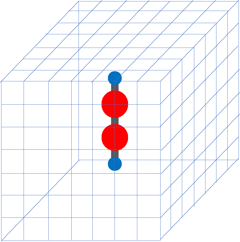
Acetylene molecule is a linear chain molecule composed of two Carbon atoms and two Hydrogen atoms.

In SALMON, we use a three-dimensional (3D) uniform grid system to express physical quantities such as electron orbitals.
Input files
To run the code, following files in the directory SALMON/samples/exercise_01_C2H2_gs/ are used:
file name |
description |
C2H2_gs.inp |
input file that contains input keywords and their values |
C_rps.dat |
pseodupotential file for carbon atom |
H_rps.dat |
pseudopotential file for hydrogen atom |
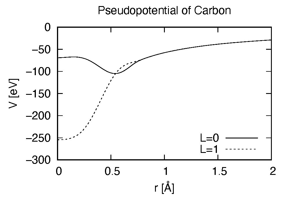
Pseudopotential files are needed for two elements, Carbon (C) and Hydrogen (H). The pseudopoential depends on the angular momentum, and looks as follows (for Carbon).
In the input file C2H2_gs.inp, input keywords are specified. Most of them are mandatory to execute the ground state calculation. This will help you to prepare an input file for other systems that you want to calculate. A complete list of the input keywords that can be used in the input file can be found in List of input keywords.
!########################################################################################!
! Excercise 01: Ground state of C2H2 molecule                                            !
!----------------------------------------------------------------------------------------!
! * The detail of this excercise is expained in our manual(see chapter: 'Exercises').    !
!   The manual can be obtained from: https://salmon-tddft.jp/documents.html              !
! * Input format consists of group of keywords like:                                     !
!     &group                                                                             !
!       input keyword = xxx                                                              !
!     /                                                                                  !
!   (see chapter: 'List of input keywords' in the manual)                                !
!----------------------------------------------------------------------------------------!
! * Conversion from unit_system = 'a.u.' to 'A_eV_fs':                                   !
!   Length: 1 [a.u.] = 0.52917721067    [Angstrom]                                       !
!   Energy: 1 [a.u.] = 27.21138505      [eV]                                             !
!   Time  : 1 [a.u.] = 0.02418884326505 [fs]                                             !
!########################################################################################!

&calculation
  !type of theory
  theory = 'dft'
/
&control
  !common name of output files
  sysname = 'C2H2'
/
&units
  !units used in input and output files
  unit_system = 'A_eV_fs'
/
&system
  !periodic boundary condition
  yn_periodic = 'n'

  !number of elements, atoms, electrons and states(orbitals)
  nelem  = 2
  natom  = 4
  nelec  = 10
  nstate = 6
/
&pseudo
  !name of input pseudo potential file
  file_pseudo(1) = './C_rps.dat'
  file_pseudo(2) = './H_rps.dat'

  !atomic number of element
  izatom(1) = 6
  izatom(2) = 1

  !angular momentum of pseudopotential that will be treated as local
  lloc_ps(1) = 1
  lloc_ps(2) = 0
  !--- Caution ---------------------------------------!
  ! Indices must correspond to those in &atomic_coor. !
  !---------------------------------------------------!
/
&functional
  !functional('PZ' is Perdew-Zunger LDA: Phys. Rev. B 23, 5048 (1981).)
  xc = 'PZ'
/
&rgrid
  !spatial grid spacing(x,y,z)
  dl(1:3) = 0.25d0, 0.25d0, 0.25d0

  !number of spatial grids(x,y,z)
  num_rgrid(1:3) = 64, 64, 64
/
&scf
  !maximum number of scf iteration and threshold of convergence
  nscf      = 300
  threshold = 1.0d-9
/
&analysis
  !output of all orbitals, density,
  !density of states, projected density of states,
  !and electron localization function
  yn_out_psi  = 'y'
  yn_out_dns  = 'y'
  yn_out_dos  = 'y'
  yn_out_pdos = 'y'
  yn_out_elf  = 'y'
/
&atomic_coor
  !cartesian atomic coodinates
  'C'    0.000000    0.000000    0.599672  1
  'H'    0.000000    0.000000    1.662257  2
  'C'    0.000000    0.000000   -0.599672  1
  'H'    0.000000    0.000000   -1.662257  2
  !--- Format ---------------------------------------------------!
  ! 'symbol' x y z index(correspond to that of pseudo potential) !
  !--------------------------------------------------------------!
/
Execusion
In a multiprocess environment, calculation will be executed as
$ mpiexec -n NPROC salmon < C2H2_gs.inp > C2H2_gs.out
where NPROC is the number of MPI processes. A standard output will be stored in the file C2H2_gs.out.
Output files
After the calculation, following output files and a directory are created in the directory that you run the code in addition to the standard output file,
name |
description |
C2H2_info.data |
information on ground state solution |
C2H2_eigen.data |
orbital energies |
C2H2_k.data |
k-point distribution (for isolated systems, only gamma point is described) |
data_for_restart |
directory where files used in the real-time calculation are contained |
psi_ob1.cube, psi_ob2.cube, ... |
electron orbitals |
dns.cube |
a cube file for electron density |
dos.data |
density of states |
pdos1.data, pdos2.data, ... |
projected density of states |
elf.cube |
electron localization function (ELF) |
PS_C_KY_n.dat |
information on pseodupotential file for carbon atom |
PS_H_KY_n.dat |
information on pseodupotential file for hydrogen atom |
We first explain the standard output file. In the beginning of the file, input variables used in the calculation are shown.
##############################################################################
# SALMON: Scalable Ab-initio Light-Matter simulator for Optics and Nanoscience
#
#                             Version 2.0.1
#
##############################################################################
  Libxc: [disabled]
   theory= dft
   use of real value orbitals =  T
 ======
 MPI distribution:
   nproc_k     :           1
   nproc_ob    :           1
   nproc_rgrid :           1           1           2
 OpenMP parallelization:
   number of threads :         256
 .........
After that, the SCF loop starts. At each iteration step, the total energy as well as orbital energies and some other quantities are displayed.
-----------------------------------------------
iter=     1     Total Energy=      -197.59254070     Gap=   -20.17834599     Vh iter= 234
    1       -29.9707      2       -28.3380      3       -13.0123      4         5.8457
    5        -9.9213      6       -14.3326
iter and int_x|rho_i(x)-rho_i-1(x)|dx/nelec        =      1 0.31853198E+00
Ne=   10.0000000000000
-----------------------------------------------
iter=     2     Total Energy=      -280.97950515     Gap=    -9.59770609     Vh iter= 247
    1       -17.4334      2       -24.4941      3       -20.1872      4         0.8020
    5        -3.4058      6        -8.7957
iter and int_x|rho_i(x)-rho_i-1(x)|dx/nelec        =      2 0.54493263E+00
Ne=   10.0000000000000
-----------------------------------------------
iter=     3     Total Energy=      -295.67034640     Gap=    -6.90359156     Vh iter= 229
    1       -16.0251      2       -19.7759      3       -17.6765      4        -0.9015
    5        -2.9323      6        -7.8050
iter and int_x|rho_i(x)-rho_i-1(x)|dx/nelec        =      3 0.13010987E+00
Ne=   10.0000000000000
When the convergence criterion is satisfied, the SCF calculation ends.
-----------------------------------------------
iter=   162     Total Energy=      -339.69525272     Gap=     6.78870999     Vh iter=   1
    1       -18.4106      2       -13.9966      3       -12.4163      4        -7.3386
    5        -7.3386      6        -0.5498
iter and int_x|rho_i(x)-rho_i-1(x)|dx/nelec        =    162 0.50237787E-08
Ne=   9.99999999999999
-----------------------------------------------
iter=   163     Total Energy=      -339.69525269     Gap=     6.78870999     Vh iter=   1
    1       -18.4106      2       -13.9966      3       -12.4163      4        -7.3386
    5        -7.3386      6        -0.5498
iter and int_x|rho_i(x)-rho_i-1(x)|dx/nelec        =    163 0.69880308E-09
Ne=   9.99999999999999
 #GS converged at   164  : 0.69880308E-09
Next, the force acting on ions and some other information related to orbital energies are shown.
===== force =====
    1 -0.33652081E-05  0.16854696E-04 -0.59496450E+00
    2 -0.59222259E-06  0.24915590E-05  0.57651725E+00
    3 -0.37839836E-05  0.20304090E-04  0.59493028E+00
    4 -0.86779607E-06  0.39560274E-05 -0.57651738E+00
orbital energy information-------------------------------
Lowest occupied orbital -0.676576619015730
Highest occupied orbital (HOMO) -0.269686750876529
Lowest unoccupied orbital (LUMO) -2.020624936948345E-002
Highest unoccupied orbital -2.020624936948345E-002
HOMO-LUMO gap  0.249480501507045
Physicaly upper bound of eps(omega)  0.656370369646246
---------------------------------------------------------
Lowest occupied orbital[eV]  -18.4105868958642
Highest occupied orbital (HOMO)[eV]  -7.33855002098465
Lowest unoccupied orbital (LUMO)[eV] -0.549840032009334
Highest unoccupied orbital[eV] -0.549840032009334
HOMO-LUMO gap[eV]   6.78870998897532
Physicaly upper bound of eps(omega)[eV]   17.8607468638548
---------------------------------------------------------
 writing restart data...
 writing completed.
In the directory data_for_restart, files that will be used in the next-step
time evolution calculations are stored.
Other output files include following information.
C2H2_info.data
Calculated orbital and total energies as well as parameters specified in the input file are shown.
C2H2_eigen.data
Orbital energies.
#esp: single-particle energies (eigen energies)
#occ: occupation numbers, io: orbital index
# 1:io, 2:esp[eV], 3:occ
C2H2_k.data
k-point distribution(for isolated systems, only gamma point is described).
# ik: k-point index
# kx,ky,kz: Reduced coordinate of k-points
# wk: Weight of k-point
# 1:ik[none] 2:kx[none] 3:ky[none] 4:kz[none] 5:wk[none]
# coefficients (2*pi/a [a.u.]) in kx, ky, kz
psi_ob1.cube, psi_ob2.cube, ...
Cube files for electron orbitals. The number in the filename indicates the index of the orbital. Atomic unit is adopted in all cube files.
dns.cube
A cube file for electron density.
dos.data
A file for density of states. The units used in this file are affected
by the input parameter, unit_system in &unit.
elf.cube
A cube file for electron localization function (ELF).
We show several image that are created from the output files.
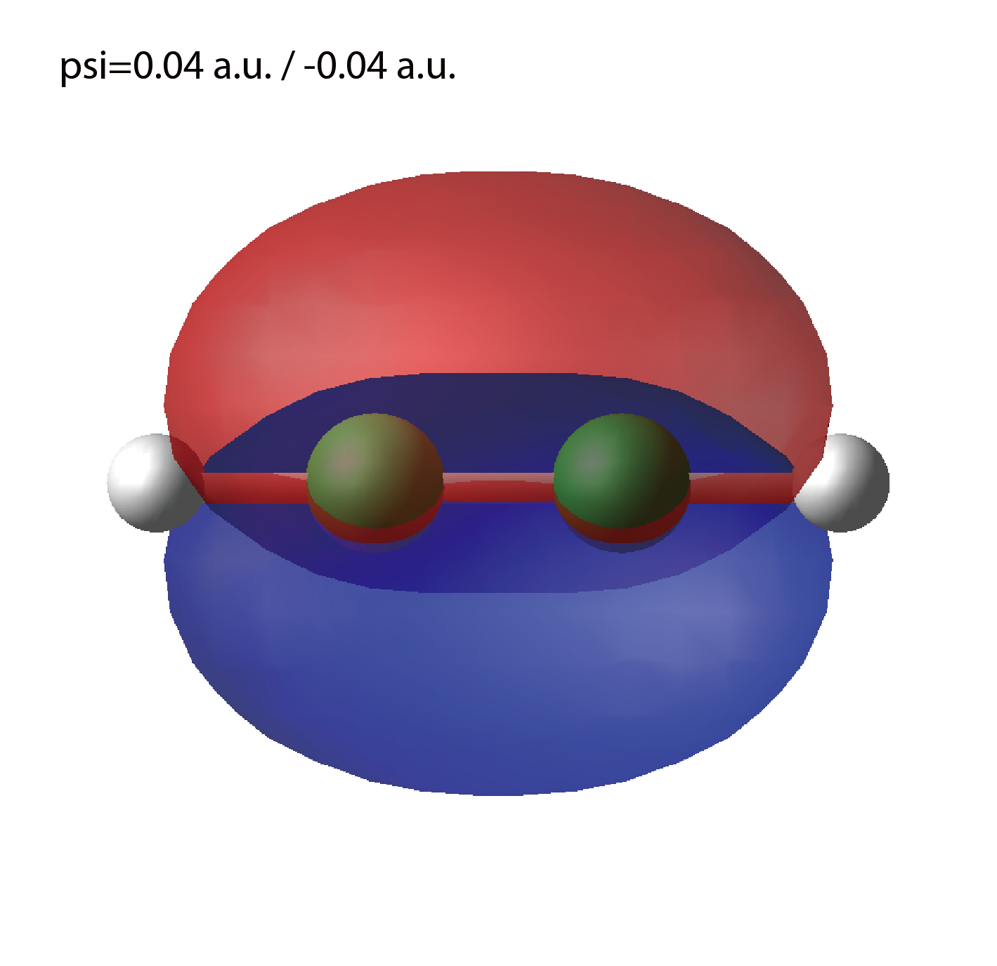
Highest occupied molecular orbital (HOMO)
The output files psi_ob1.cube, psi_ob2.cube, ... are used to create the image.
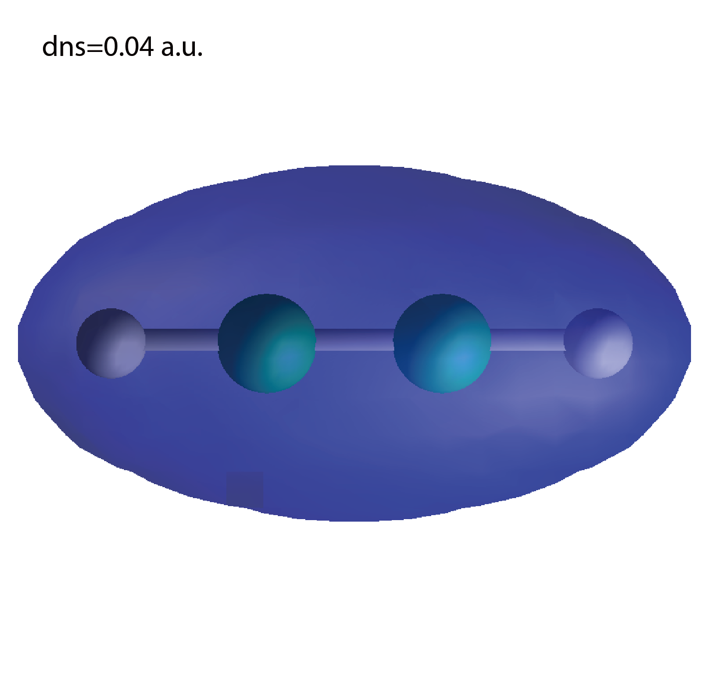
Electron density
The output files dns.cube, ... are used to create the image.
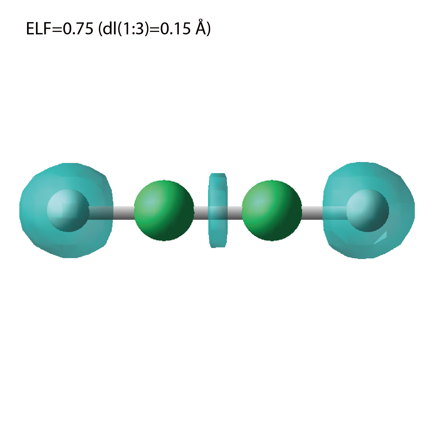
Electron localization function
The output files elf.cube, ... are used to create the image.
Exercise-2: Polarizability and photoabsorption of C2H2 molecule
In this exercise, we learn the linear response calculation in the acetylene (C2H2) molecule, solving the time-dependent Kohn-Sham equation. The linear response calculation provides the polarizability and the oscillator strength distribution of the molecule. This exercise should be carried out after finishing the ground state calculation that was explained in Exercise-1.
Polarizability  is the basic quantity
that characterizes optical responses of molecules and nano-particles,
where
is the basic quantity
that characterizes optical responses of molecules and nano-particles,
where  indicate Cartesian components,
  .
The polarizability relates the
.
The polarizability relates the  component of the electric dipole moment at time
  ,
,  ,
with the
,
with the  component of the electric field at time
  ,
,

We introduce a frequency-dependent polarizability by the time-frequency Fourier transformation of the polarizability,
The imaginary part of the frequency-dependent polarizability is
related to the photoabsorption cross section  by
by
The photoabsorption cross section is also related to the oscillator strength distribution by
In SALMON, the polarizability is calculated in time domain.
First the ground state orbital  that
satisfies the Kohn-Sham equation,
that
satisfies the Kohn-Sham equation,
is prepared. Then an impulsive force given by the potential
is applied to all electrons in the C2H2 molecule along the molecular axis
which we take  axis.
axis.  is the magnitude of the impulse,
and
is the magnitude of the impulse,
and  is the Dirac's delta function.
The orbital is distorted by the impulsive force at
is the Dirac's delta function.
The orbital is distorted by the impulsive force at  .
Immediately after the impulse is applied, the orbital becomes
.
Immediately after the impulse is applied, the orbital becomes

After the impulsive force is applied at ,
a time evolution calculation is carried out without any external fields,
During the time evolution, the electric dipole moment given by

is monitored. After the time evolution calculation, a time-frequency Fourier transformation is carried out for the electric dipole moment to obtain the frequency-dependent polarizability by
Input files
To run the code, following files are necessary:
file name |
description |
C2H2_rt_response.inp |
input file that contain input keywords and their values. |
C_rps.dat |
pseodupotential file for carbon |
H_rps.dat |
pseudopotential file for hydrogen |
restart |
directory created in the ground state calculation
(rename the directory from data_for_restart to restart)
|
First three files are prepared in the directory SALMON/samples/exercise_02_C2H2_lr/.
The file C2H2_rt_response.inp that contains input keywords and their values.
The pseudopotential files should be the same as those used in the ground state calculation.
In the directory restart, those files created in the ground state calculation and stored
in the directory data_for_restart are included.
Therefore, copy the directory as cp -R data_for_restart restart
if you calculate at the same directory as you did the ground state calculation.
In the input file C2H2_rt_response.inp, input keywords are specified. Most of them are mandatory to execute the linear response calculation. This will help you to prepare the input file for other systems that you want to calculate. A complete list of the input keywords that can be used in the input file can be found in List of input keywords.
!########################################################################################!
! Excercise 02: Polarizability and photoabsorption of C2H2 molecule                      !
!----------------------------------------------------------------------------------------!
! * The detail of this excercise is expained in our manual(see chapter: 'Exercises').    !
!   The manual can be obtained from: https://salmon-tddft.jp/documents.html              !
! * Input format consists of group of keywords like:                                     !
!     &group                                                                             !
!       input keyword = xxx                                                              !
!     /                                                                                  !
!   (see chapter: 'List of input keywords' in the manual)                                !
!----------------------------------------------------------------------------------------!
! * Conversion from unit_system = 'a.u.' to 'A_eV_fs':                                   !
!   Length: 1 [a.u.] = 0.52917721067    [Angstrom]                                       !
!   Energy: 1 [a.u.] = 27.21138505      [eV]                                             !
!   Time  : 1 [a.u.] = 0.02418884326505 [fs]                                             !
!----------------------------------------------------------------------------------------!
! * Copy the ground state data directory('data_for_restart') (or make symbolic link)     !
!   calculated in 'samples/exercise_01_C2H2_gs/' and rename the directory to 'restart/'  !
!   in the current directory.                                                            !
!########################################################################################!

&calculation
  !type of theory
  theory = 'tddft_response'
/
&control
  !common name of output files
  sysname = 'C2H2'
/
&units
  !units used in input and output files
  unit_system = 'A_eV_fs'
/
&system
  !periodic boundary condition
  yn_periodic = 'n'

  !number of elements, atoms, electrons and states(orbitals)
  nelem  = 2
  natom  = 4
  nelec  = 10
  nstate = 6
/
&pseudo
  !name of input pseudo potential file
  file_pseudo(1) = './C_rps.dat'
  file_pseudo(2) = './H_rps.dat'

  !atomic number of element
  izatom(1) = 6
  izatom(2) = 1

  !angular momentum of pseudopotential that will be treated as local
  lloc_ps(1) = 1
  lloc_ps(2) = 0
  !--- Caution ---------------------------------------!
  ! Indices must correspond to those in &atomic_coor. !
  !---------------------------------------------------!
/
&functional
  !functional('PZ' is Perdew-Zunger LDA: Phys. Rev. B 23, 5048 (1981).)
  xc = 'PZ'
/
&rgrid
  !spatial grid spacing(x,y,z)
  dl(1:3) = 0.25d0, 0.25d0, 0.25d0

  !number of spatial grids(x,y,z)
  num_rgrid(1:3) = 64, 64, 64
/
&tgrid
  !time step size and number of time grids(steps)
  dt = 1.25d-3
  nt = 5000
/
&emfield
  !envelope shape of the incident pulse('impulse': impulsive field)
  ae_shape1 = 'impulse'

  !polarization unit vector(real part) for the incident pulse(x,y,z)
  epdir_re1(1:3) = 0.0d0, 0.0d0, 1.0d0
  !--- Caution ---------------------------------------------------------!
  ! Defenition of the incident pulse is wrriten in:                     !
  ! https://www.sciencedirect.com/science/article/pii/S0010465518303412 !
  !---------------------------------------------------------------------!
/
as_shape1='impulse' is used. It indicates that a weak impulsive perturbation is applied at .&analysis
!energy grid size and number of energy grids for output files
de = 1.0d-2
nenergy = 3000
/
&atomic_coor
  !cartesian atomic coodinates
  'C'    0.000000    0.000000    0.599672  1
  'H'    0.000000    0.000000    1.662257  2
  'C'    0.000000    0.000000   -0.599672  1
  'H'    0.000000    0.000000   -1.662257  2
  !--- Format ---------------------------------------------------!
  ! 'symbol' x y z index(correspond to that of pseudo potential) !
  !--------------------------------------------------------------!
/
Execusion
Before execusion, remember to copy the directory restart that is created in the ground state calculation as data_for_restart in the present directory. In a multiprocess environment, calculation will be executed as
$ mpiexec -n NPROC salmon < C2H2_rt_response.inp > C2H2_rt_response.out
where NPROC is the number of MPI processes. A standard output will be stored in the file C2H2_rt_response.out.
Output files
After the calculation, following output files are created in the directory that you run the code,
file name |
description |
C2H2_response.data |
polarizability and oscillator strength distribution as functions of energy |
C2H2_rt.data |
components of
change of dipole moment
(electrons/plus definition)
and total dipole moment
(electrons/minus + ions/plus)
as functions of time
|
C2H2_rt_energy.data |
components of total energy and difference of total energy as functions of time |
PS_C_KY_n.dat |
information on pseodupotential file for carbon atom |
PS_H_KY_n.dat |
information on pseodupotential file for hydrogen atom |
We first explain the standard output file. In the beginning of the file, input variables used in the calculation are shown.
##############################################################################
# SALMON: Scalable Ab-initio Light-Matter simulator for Optics and Nanoscience
#
#                             Version 2.0.1
##############################################################################
  Libxc: [disabled]
   theory= tddft_response

 Total time step      =        5000
 Time step[fs]        =  1.250000000000000E-003
 Energy range         =        3000
 Energy resolution[eV]=  1.000000000000000E-002
 Field strength[a.u.] =  1.000000000000000E-002
   use of real value orbitals =  F
 ======
 .........
After that, the time evolution loop starts. At every 10 iteration steps, the time, dipole moments in three Cartesian directions, the total number of electrons, the total energy, and the number of iterations solving the Poisson equation are displayed.
 time-step    time[fs]                           Dipole moment(xyz)[A]      electrons  Total energy[eV]    iterVh
#----------------------------------------------------------------------
      10    0.01250000 -0.56521137E-07 -0.28812833E-07 -0.25558983E-01    10.00000000     -339.68150366   34
      20    0.02500000 -0.19835467E-06 -0.10147641E-06 -0.45169126E-01     9.99999999     -339.68147442   49
      30    0.03750000 -0.37937911E-06 -0.19537418E-06 -0.57843871E-01     9.99999999     -339.68146891   45
      40    0.05000000 -0.56465010E-06 -0.29324906E-06 -0.64072126E-01     9.99999999     -339.68146804   38
      50    0.06250000 -0.73343753E-06 -0.38431758E-06 -0.65208422E-01     9.99999999     -339.68146679   25
      60    0.07500000 -0.87559727E-06 -0.46276791E-06 -0.62464066E-01     9.99999999     -339.68146321   35
      70    0.08750000 -0.98769124E-06 -0.52594670E-06 -0.56740338E-01     9.99999998     -339.68145535   20
      80    0.10000000 -0.10701350E-05 -0.57309375E-06 -0.48483747E-01     9.99999998     -339.68144840   40
      90    0.11250000 -0.11253992E-05 -0.60455485E-06 -0.38296037E-01     9.99999998     -339.68144186   21
Explanations of other output files are given below:
C2H2_rt.data
Results of time evolution calculation for vector potential, electric field, and dipole moment. In the first several lines, explanations of included data are given.
# Real time calculation:
# Ac_ext: External vector potential field
# E_ext: External electric field
# Ac_tot: Total vector potential field
# E_tot: Total electric field
# ddm_e: Change of dipole moment (electrons/plus definition)
# dm: Total dipole moment (electrons/minus + ions/plus)
# 1:Time[fs] 2:Ac_ext_x[fs*V/Angstrom] 3:Ac_ext_y[fs*V/Angstrom] 4:Ac_ext_z[fs*V/Angstrom] 5:E_ext_x[V/Angstrom] 6:E_ext_y[V/Angstrom] 7:E_ext_z[V/Angstrom] 8:Ac_tot_x[fs*V/Angstrom] 9:Ac_tot_y[fs*V/Angstrom] 10:Ac_tot_z[fs*V/Angstrom] 11:E_tot_x[V/Angstrom] 12:E_tot_y[V/Angstrom] 13:E_tot_z[V/Angstrom] 14:ddm_e_x[Angstrom] 15:ddm_e_y[Angstrom] 16:ddm_e_z[Angstrom] 17:dm_x[Angstrom] 18:dm_y[Angstrom] 19:dm_z[Angstrom]
Using first column (time in femtosecond) and 19th column (dipole moment in direction),
the following graph can be drawn.
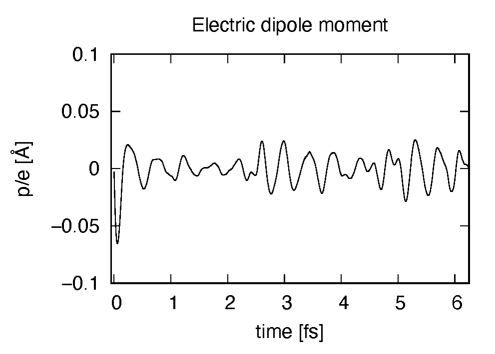
The dipole moment shows oscillations in femtosecond time scale that reflec electronic excitations.
C2H2_response.data
Time-frequency Fourier transformation of the dipole moment gives the polarizability and the strength function.
# Fourier-transform spectra:
# alpha: Polarizability
# df/dE: Strength function
# 1:Energy[eV] 2:Re(alpha_x)[Augstrom^2/V] 3:Re(alpha_y)[Augstrom^2/V] 4:Re(alpha_z)[Augstrom^2/V] 5:Im(alpha_x)[Augstrom^2/V] 6:Im(alpha_y)[Augstrom^2/V] 7:Im(alpha_z)[Augstrom^2/V] 8:df_x/dE[none] 9:df_y/dE[none] 10:df_z/dE[none]
Using first column (energy in electron-volt) and 10th column (oscillator strength distribution in direction),
the following graph can be drawn.
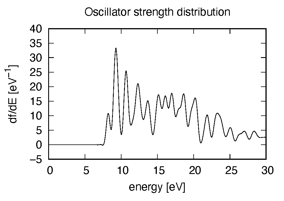
There appears many peaks above the HOMO-LUMO gap energy. The strong excitation appears at around 9.3 eV.
C2H2_rt_energy.data
Energies are stored as functions of time.
# Real time calculation:
# Eall: Total energy
# Eall0: Initial energy
# 1:Time[fs] 2:Eall[eV] 3:Eall-Eall0[eV]
Eall and Eall-Eall0 are total energy and electronic excitation energy, respectively.
Exercise-3: Electron dynamics in C2H2 molecule under a pulsed electric field
In this exercise, we learn the calculation of the electron dynamics in the acetylene (C2H2) molecule under a pulsed electric field, solving the time-dependent Kohn-Sham equation. As outputs of the calculation, such quantities as the total energy and the electric dipole moment of the system as functions of time are calculated. This tutorial should be carried out after finishing the ground state calculation that was explained in Exercise-1.
In the calculation, a pulsed electric field specified by the following vector potential will be used,

The electric field is given by  .
The parameters that characterize the pulsed field such as the amplitude
.
The parameters that characterize the pulsed field such as the amplitude  ,
frequency
,
frequency  , pulse duration
  , polarization direction
  ,
are specified in the input file.
In the time dependent Kohn-Sham equation, the external field is included as
the scalar potential,
,
are specified in the input file.
In the time dependent Kohn-Sham equation, the external field is included as
the scalar potential,  .
.
Input files
To run the code, following files are necessary:
file name |
description |
C2H2_rt_pulse.inp |
input file that contain input keywords and their values. |
C_rps.dat |
pseodupotential file for carbon |
H_rps.dat |
pseudopotential file for hydrogen |
restart |
directory created in the ground state calculation
(rename the directory from data_for_restart to restart)
|
First three files are prepared in the directory SALMON/samples/exercise_03_C2H2_rt/.
The file C2H2_rt_pulse.inp that contains input keywords and their values.
The pseudopotential files should be the same as those used in the ground state calculation.
In the directory restart, those files created in the ground state calculation and stored
in the directory data_for_restart are included.
Therefore, copy the directory as cp -R data_for_restart restart
if you calculate at the same directory as you did the ground state calculation.
In the input file C2H2_rt_pulse.inp, input keywords are specified. Most of them are mandatory to execute the calculation of electron dynamics induced by a pulsed electric field. This will help you to prepare the input file for other systems and other pulsed electric fields that you want to calculate. A complete list of the input keywords that can be used in the input file can be found in List of input keywords.
!########################################################################################!
! Excercise 03:  Electron dynamics in C2H2 molecule under a pulsed electric field        !
!----------------------------------------------------------------------------------------!
! * The detail of this excercise is expained in our manual(see chapter: 'Exercises').    !
!   The manual can be obtained from: https://salmon-tddft.jp/documents.html              !
! * Input format consists of group of keywords like:                                     !
!     &group                                                                             !
!       input keyword = xxx                                                              !
!     /                                                                                  !
!   (see chapter: 'List of input keywords' in the manual)                                !
!----------------------------------------------------------------------------------------!
! * Conversion from unit_system = 'a.u.' to 'A_eV_fs':                                   !
!   Length: 1 [a.u.] = 0.52917721067    [Angstrom]                                       !
!   Energy: 1 [a.u.] = 27.21138505      [eV]                                             !
!   Time  : 1 [a.u.] = 0.02418884326505 [fs]                                             !
!----------------------------------------------------------------------------------------!
! * Copy the ground state data directory('data_for_restart') (or make symbolic link)     !
!   calculated in 'samples/exercise_01_C2H2_gs/' and rename the directory to 'restart/'  !
!   in the current directory.                                                            !
!########################################################################################!

&calculation
  !type of theory
  theory = 'tddft_pulse'
/
&control
  !common name of output files
  sysname = 'C2H2'
/
&units
  !units used in input and output files
  unit_system = 'A_eV_fs'
/
&system
  !periodic boundary condition
  yn_periodic = 'n'

  !number of elements, atoms, electrons and states(orbitals)
  nelem  = 2
  natom  = 4
  nelec  = 10
  nstate = 6
/
&pseudo
  !name of input pseudo potential file
  file_pseudo(1) = './C_rps.dat'
  file_pseudo(2) = './H_rps.dat'

  !atomic number of element
  izatom(1) = 6
  izatom(2) = 1

  !angular momentum of pseudopotential that will be treated as local
  lloc_ps(1) = 1
  lloc_ps(2) = 0
  !--- Caution ---------------------------------------!
  ! Indices must correspond to those in &atomic_coor. !
  !---------------------------------------------------!
/
&functional
  !functional('PZ' is Perdew-Zunger LDA: Phys. Rev. B 23, 5048 (1981).)
  xc = 'PZ'
/
&rgrid
  !spatial grid spacing(x,y,z)
  dl(1:3) = 0.25d0, 0.25d0, 0.25d0

  !number of spatial grids(x,y,z)
  num_rgrid(1:3) = 64, 64, 64
/
&tgrid
  !time step size and number of time grids(steps)
  dt = 1.25d-3
  nt = 5000
/
&emfield
  !envelope shape of the incident pulse('Ecos2': cos^2 type envelope for scalar potential)
  ae_shape1 = 'Acos2'

  !peak intensity(W/cm^2) of the incident pulse
  I_wcm2_1 = 5.00d13

  !duration of the incident pulse
  tw1 = 6.00d0

  !mean photon energy(average frequency multiplied by the Planck constant) of the incident pulse
  omega1 = 3.10d0

  !polarization unit vector(real part) for the incident pulse(x,y,z)
  epdir_re1(1:3) = 0.00d0, 0.00d0, 1.00d0
  !--- Caution ---------------------------------------------------------!
  ! Defenition of the incident pulse is wrriten in:                     !
  ! https://www.sciencedirect.com/science/article/pii/S0010465518303412 !
  !---------------------------------------------------------------------!
/
&analysis
  !energy grid size and number of energy grids for output files
  de      = 1.0d-2
  nenergy = 10000
/
&atomic_coor
  !cartesian atomic coodinates
  'C'    0.000000    0.000000    0.599672  1
  'H'    0.000000    0.000000    1.662257  2
  'C'    0.000000    0.000000   -0.599672  1
  'H'    0.000000    0.000000   -1.662257  2
  !--- Format ---------------------------------------------------!
  ! 'symbol' x y z index(correspond to that of pseudo potential) !
  !--------------------------------------------------------------!
/
Execusion
Before execusion, remember to copy the directory restart that is created in the ground state calculation as data_for_restart in the present directory. In a multiprocess environment, calculation will be executed as
$ mpiexec -n NPROC salmon < C2H2_rt_pulse.inp > C2H2_rt_pulse.out
where NPROC is the number of MPI processes. A standard output will be stored in the file C2H2_rt_pulse.out.
Output files
After the calculation, following output files are created in the directory that you run the code,
file name |
description |
C2H2_pulse.data |
dipole moment as functions of energy |
C2H2_rt.data |
components of
change of dipole moment
(electrons/plus definition)
and total dipole moment
(electrons/minus + ions/plus)
as functions of time
|
C2H2_rt_energy.data |
components of total energy and difference of total energy as functions of time |
PS_C_KY_n.dat |
information on pseodupotential file for carbon atom |
PS_H_KY_n.dat |
information on pseodupotential file for hydrogen atom |
We first explain the standard output file. In the beginning of the file, input variables used in the calculation are shown.
##############################################################################
# SALMON: Scalable Ab-initio Light-Matter simulator for Optics and Nanoscience
#
#                             Version 2.0.1
##############################################################################
  Libxc: [disabled]
   theory= tddft_pulse

 Total time step      =        5000
 Time step[fs]        =  1.250000000000000E-003
 Energy range         =       10000
 Energy resolution[eV]=  1.000000000000000E-002
Laser frequency     = 3.10[eV]
Pulse width of laser=      6.00000000[fs]
Laser intensity     =  0.50000000E+14[W/cm^2]
   use of real value orbitals =  F
 ======
 ........
After that, the time evolution loop starts. At every 10 iteration steps, the time, dipole moments in three Cartesian directions, the total number of electrons, the total energy, and the number of iterations solving the Poisson equation are displayed.
 time-step    time[fs]                           Dipole moment(xyz)[A]      electrons  Total energy[eV]    iterVh
#----------------------------------------------------------------------
      10    0.01250000 -0.57275542E-07 -0.29197105E-07 -0.74600728E-06    10.00000000     -339.69524047    1
      20    0.02500000 -0.20616352E-06 -0.10537273E-06 -0.10256205E-04    10.00000000     -339.69524348    1
      30    0.03750000 -0.40063325E-06 -0.20597522E-06 -0.47397133E-04    10.00000000     -339.69524090    3
      40    0.05000000 -0.59093535E-06 -0.30630513E-06 -0.13774845E-03    10.00000000     -339.69524287    1
      50    0.06250000 -0.75588343E-06 -0.39552925E-06 -0.31097825E-03    10.00000000     -339.69523949    5
      60    0.07500000 -0.89221538E-06 -0.47142217E-06 -0.59735355E-03    10.00000000     -339.69523784   11
      70    0.08750000 -0.99769538E-06 -0.53192187E-06 -0.10253308E-02    10.00000000     -339.69523285    5
      80    0.10000000 -0.10738281E-05 -0.57676878E-06 -0.16195168E-02     9.99999999     -339.69522482   19
      90    0.11250000 -0.11250289E-05 -0.60722757E-06 -0.23985719E-02     9.99999999     -339.69521092    2
Explanations of the files are given below:
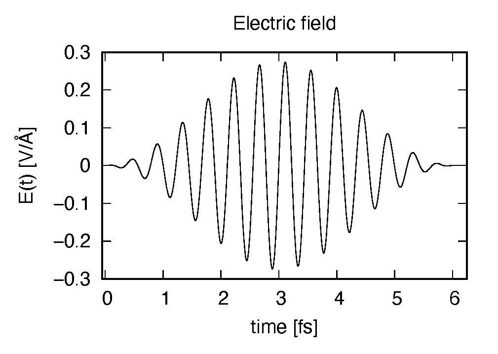
C2H2_rt.data
Results of time evolution calculation for vector potential, electric field, and dipole moment. In the first several lines, explanations of data included data are given.
# Real time calculation:
# Ac_ext: External vector potential field
# E_ext: External electric field
# Ac_tot: Total vector potential field
# E_tot: Total electric field
# ddm_e: Change of dipole moment (electrons/plus definition)
# dm: Total dipole moment (electrons/minus + ions/plus)
# 1:Time[fs] 2:Ac_ext_x[fs*V/Angstrom] 3:Ac_ext_y[fs*V/Angstrom] 4:Ac_ext_z[fs*V/Angstrom] 5:E_ext_x[V/Angstrom] 6:E_ext_y[V/Angstrom] 7:E_ext_z[V/Angstrom] 8:Ac_tot_x[fs*V/Angstrom] 9:Ac_tot_y[fs*V/Angstrom] 10:Ac_tot_z[fs*V/Angstrom] 11:E_tot_x[V/Angstrom] 12:E_tot_y[V/Angstrom] 13:E_tot_z[V/Angstrom] 14:ddm_e_x[Angstrom] 15:ddm_e_y[Angstrom] 16:ddm_e_z[Angstrom] 17:dm_x[Angstrom] 18:dm_y[Angstrom] 19:dm_z[Angstrom]
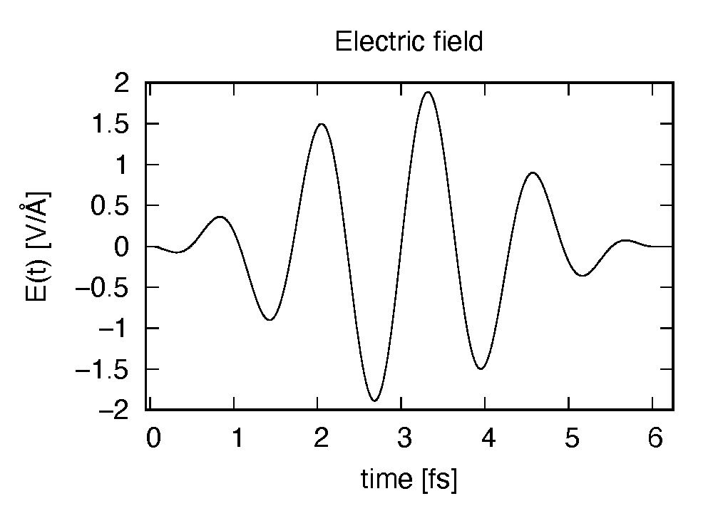
The applied electric field is drawn using the first column (time in femtosecond) and the 7th column
(electric field in direction in Volt per Angstrom).
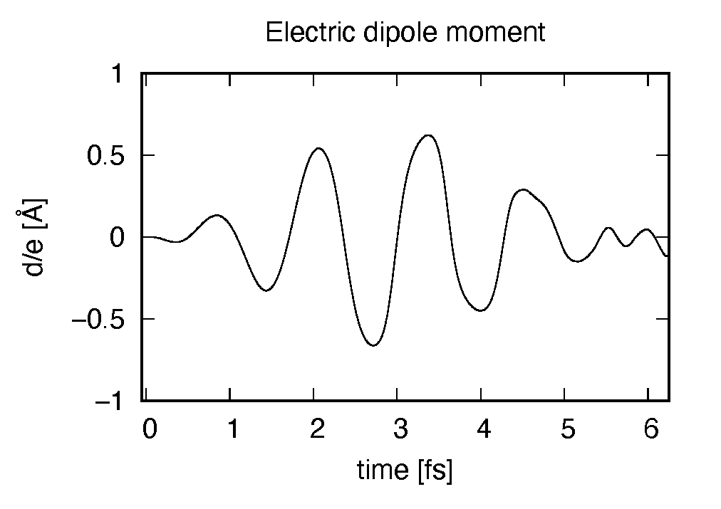
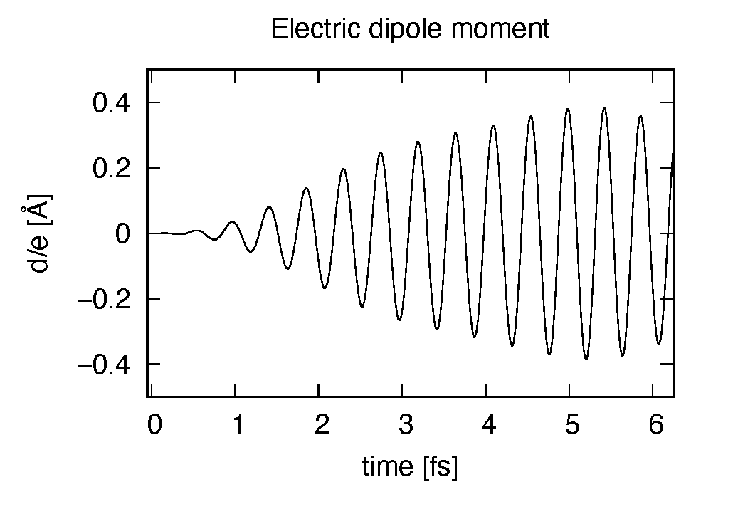
The induced dipole moment is drawn using the first column (time in femtosecond) and 19th column
(dipole moment in direction).
It shows an oscillation similar to the applied electric field. However, the response is not linear
since the applied electric field is rather strong.
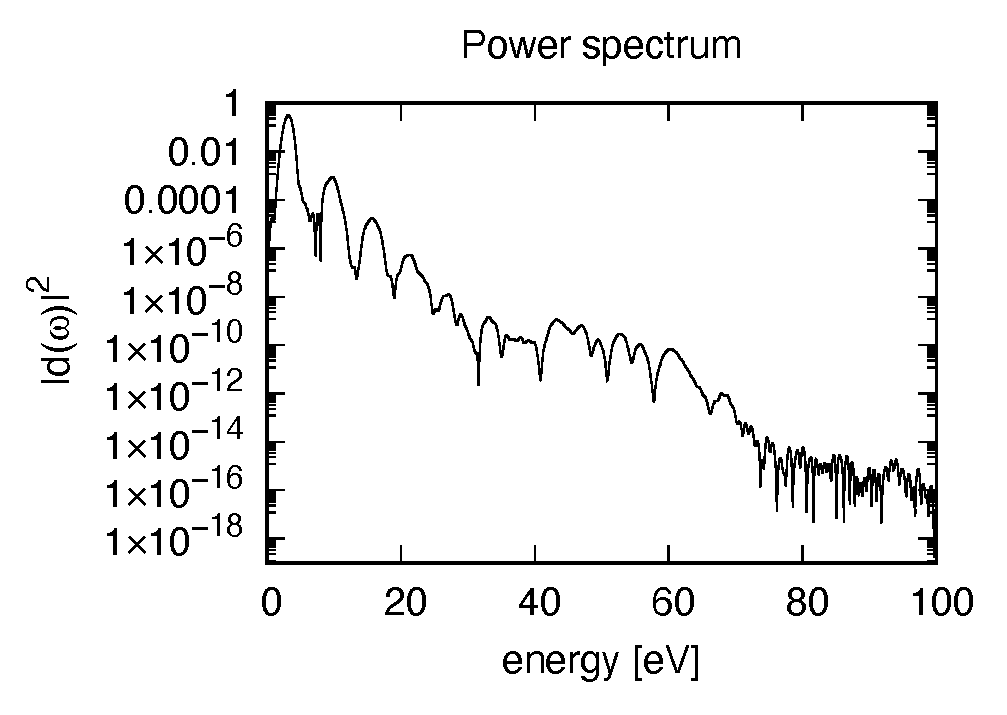
C2H2_pulse.data
Time-frequency Fourier transformation of the dipole moment. In the first several lines, explanations of data included data are given.
# Fourier-transform spectra:
# energy: Frequency
# dm: Dopile moment
# 1:energy[eV] 2:Re(dm_x)[fs*Angstrom] 3:Re(dm_y)[fs*Angstrom] 4:Re(dm_z)[fs*Angstrom] 5:Im(dm_x)[fs*Angstrom] 6:Im(dm_y)[fs*Angstrom] 7:Im(dm_z)[fs*Angstrom] 8:|dm_x|^2[fs^2*Angstrom^2] 9:|dm_y|^2[fs^2*Angstrom^2] 10:|dm_z|^2[fs^2*Angstrom^2]
The spectrum of the induced dipole moment,  is shown in logarithmic scale as a function
of the energy,
is shown in logarithmic scale as a function
of the energy,  . High harmonic generations are visible in the spectrum.
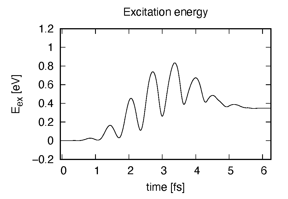
C2H2_rt_energy.data
Energies are stored as functions of time. In the first several lines, explanations of data included data are given.
# Real time calculation:
# Eall: Total energy
# Eall0: Initial energy
# 1:Time[fs] 2:Eall[eV] 3:Eall-Eall0[eV]
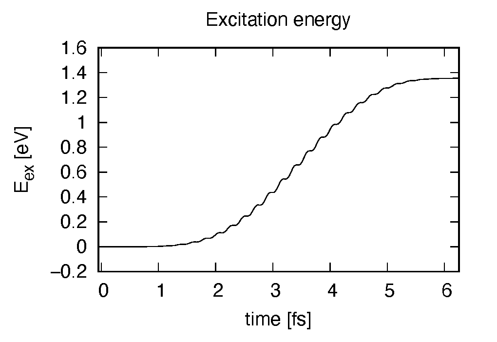
Eall and Eall-Eall0 are total energy and electronic excitation energy, respectively. The figure below shows the electronic excitation energy as a function of time, using the first column (time in femtosecond) and the 3rd column (Eall-Eall0). Although the frequency is below the HOMO-LUMO gap energy, electronic excitations take place because of nonlinear absorption process.
Additional exercise
If we change parameters of the applied electric field, we find a drastic change
in the electronic excitations. In the example below, we increase the intensity
from I_wcm2_1 = 5.00d13 to I_wcm2_1 = 1.00d12 and changes the frequency
from omega1 = 3.10d0 to omega1 = 9.28d0. The new frequency corresponds
to the resonant excitation energy seen in the linear response analysis shown in
in Exercise-2.
The change in the input file is shown below.
&emfield
  !envelope shape of the incident pulse('Ecos2': cos^2 type envelope for scalar potential)
  ae_shape1 = 'Acos2'

  !peak intensity(W/cm^2) of the incident pulse
  I_wcm2_1 = 1.00d12

  !duration of the incident pulse
  tw1 = 6.00d0

  !mean photon energy(average frequency multiplied by the Planck constant) of the incident pulse
  omega1 = 9.28d0

  !polarization unit vector(real part) for the incident pulse(x,y,z)
  epdir_re1(1:3) = 0.00d0, 0.00d0, 1.00d0
The applied electric field shows a rapid oscillation.
The induced dipole moment also shows a rapid oscillation and does not decrease even though the electric field decreases. This is because the frequency of the applied electric field coincides with the excitation energy of the molecule.
The electronic excitation energy also shows a monotonic increase. Although the strength of the applied electric field is much smaller than the previous case, the amount of the excitation energy is larger, again due to the resonant excitation.
Crystalline silicon (periodic solids)
Exercise-4: Ground state of crystalline silicon
In this exercise, we learn the the ground state calculation of the crystalline silicon of a diamond structure. Calculation is done in a cubic unit cell that contains eight silicon atoms. This exercise will be useful to learn how to set up calculations in SALMON for any periodic systems such as crystalline solid.
Input files
To run the code, following files in samples are used:
file name |
description |
Si_gs.inp |
input file that contains input keywords and their values |
Si_rps.dat |
pseodupotential file for silicon atom |
In the input file Si_gs.inp, input keywords are specified. Most of them are mandatory to execute the ground state calculation. This will help you to prepare an input file for other systems that you want to calculate. A complete list of the input keywords that can be used in the input file can be found in List of input keywords.
!########################################################################################!
! Excercise 04: Ground state of crystalline silicon(periodic solids)                     !
!----------------------------------------------------------------------------------------!
! * The detail of this excercise is expained in our manual(see chapter: 'Exercises').    !
!   The manual can be obtained from: https://salmon-tddft.jp/documents.html              !
! * Input format consists of group of keywords like:                                     !
!     &group                                                                             !
!       input keyword = xxx                                                              !
!     /                                                                                  !
!   (see chapter: 'List of input keywords' in the manual)                                !
!----------------------------------------------------------------------------------------!
! * Conversion from unit_system = 'a.u.' to 'A_eV_fs':                                   !
!   Length: 1 [a.u.] = 0.52917721067    [Angstrom]                                       !
!   Energy: 1 [a.u.] = 27.21138505      [eV]                                             !
!   Time  : 1 [a.u.] = 0.02418884326505 [fs]                                             !
!########################################################################################!

&calculation
  !type of theory
  theory = 'dft'
/
&control
  !common name of output files
  sysname = 'Si'
/
&units
  !units used in input and output files
  unit_system = 'a.u.'
/
&system
  !periodic boundary condition
  yn_periodic = 'y'

  !grid box size(x,y,z)
  al(1:3) = 10.26d0, 10.26d0, 10.26d0

  !number of elements, atoms, electrons and states(bands)
  nelem  = 1
  natom  = 8
  nelec  = 32
  nstate = 32
/
&pseudo
  !name of input pseudo potential file
  file_pseudo(1) = './Si_rps.dat'

  !atomic number of element
  izatom(1) = 14

  !angular momentum of pseudopotential that will be treated as local
  lloc_ps(1) = 2
  !--- Caution -------------------------------------------!
  ! Index must correspond to those in &atomic_red_coor.   !
  !-------------------------------------------------------!
/
&functional
  !functional('PZ' is Perdew-Zunger LDA: Phys. Rev. B 23, 5048 (1981).)
  xc = 'PZ'
/
&rgrid
  !number of spatial grids(x,y,z)
  num_rgrid(1:3) = 12, 12, 12
/
&kgrid
  !number of k-points(x,y,z)
  num_kgrid(1:3) = 4, 4, 4
/
&scf
  !maximum number of scf iteration and threshold of convergence
  nscf      = 300
  threshold = 1.0d-9
/
&atomic_red_coor
  !cartesian atomic reduced coodinates
  'Si'       .0      .0      .0      1
  'Si'       .25     .25     .25     1
  'Si'       .5      .0      .5      1
  'Si'       .0      .5      .5      1
  'Si'       .5      .5      .0      1
  'Si'       .75     .25     .75     1
  'Si'       .25     .75     .75     1
  'Si'       .75     .75     .25     1
  !--- Format ---------------------------------------------------!
  ! 'symbol' x y z index(correspond to that of pseudo potential) !
  !--------------------------------------------------------------!
/
Output files
After the calculation, following output files and a directory are created in the directory that you run the code,
name |
description |
Si_info.data |
information on ground state solution |
Si_eigen.data |
energy eigenvalues of orbitals |
Si_k.data |
k-point distribution |
PS_Si_KY_n.dat |
information on pseodupotential file for silicon atom |
data_for_restart |
directory where files used in the real-time calculation are contained |
Main results of the calculation such as orbital energies are included in Si_info.data. Explanations of the Si_info.data and other output files are below:
Si_info.data
Calculated orbital and total energies as well as parameters specified in the input file are shown in this file.
Si_eigen.data
1 particle energies.
#esp: single-particle energies (eigen energies)
#occ: occupation numbers, io: orbital index
# 1:io, 2:esp[a.u.], 3:occ
Si_k.data
k-point distribution.
# ik: k-point index
# kx,ky,kz: Reduced coordinate of k-points
# wk: Weight of k-point
# 1:ik[none] 2:kx[none] 3:ky[none] 4:kz[none] 5:wk[none]
# coefficients (2*pi/a [a.u.]) in kx, ky, kz
Exercise-5: Dielectric function of crystalline silicon
In this exercise, we learn the linear response calculation of the crystalline silicon of a diamond structure. Calculation is done in a cubic unit cell that contains eight silicon atoms. This exercise should be carried out after finishing the ground state calculation that was explained in Exercise-4. An impulsive perturbation is applied to all electrons in the unit cell along z direction. Since the dielectric function is isotropic in the diamond structure, calculated dielectric function should not depend on the direction of the perturbation. During the time evolution, electric current averaged over the unit cell volume is calculated. A time-frequency Fourier transformation of the electric current gives us a frequency-dependent conductivity. The dielectric function may be obtained from the conductivity using a standard relation.
Input files
To run the code, following files in samples are used:
file name |
description |
Si_rt_response.inp |
input file that contain input keywords and their values |
Si_rps.dat |
pseodupotential file of silicon |
restart |
directory created in the ground
state calculation
(rename the
directory from
data_for_restart to restart)
|
In the input file Si_rt_response.inp, input keywords are specified. Most of them are mandatory to execute the calculation. This will help you to prepare the input file for other systems that you want to calculate. A complete list of the input keywords can be found in List of input keywords.
!########################################################################################!
! Excercise 05: Dielectric function of crystalline silicon                               !
!----------------------------------------------------------------------------------------!
! * The detail of this excercise is expained in our manual(see chapter: 'Exercises').    !
!   The manual can be obtained from: https://salmon-tddft.jp/documents.html              !
! * Input format consists of group of keywords like:                                     !
!     &group                                                                             !
!       input keyword = xxx                                                              !
!     /                                                                                  !
!   (see chapter: 'List of input keywords' in the manual)                                !
!----------------------------------------------------------------------------------------!
! * Conversion from unit_system = 'a.u.' to 'A_eV_fs':                                   !
!   Length: 1 [a.u.] = 0.52917721067    [Angstrom]                                       !
!   Energy: 1 [a.u.] = 27.21138505      [eV]                                             !
!   Time  : 1 [a.u.] = 0.02418884326505 [fs]                                             !
!----------------------------------------------------------------------------------------!
! * Copy the ground state data directory('data_for_restart') (or make symbolic link)     !
!   calculated in 'samples/exercise_04_bulkSi_gs/' and rename the directory to 'restart/'!
!   in the current directory.                                                            !
!########################################################################################!

&calculation
  !type of theory
  theory = 'tddft_response'
/
&control
  !common name of output files
  sysname = 'Si'
/
&units
  !units used in input and output files
  unit_system = 'a.u.'
/
&system
  !periodic boundary condition
  yn_periodic = 'y'

  !grid box size(x,y,z)
  al(1:3) = 10.26d0, 10.26d0, 10.26d0

  !number of elements, atoms, electrons and states(bands)
  nelem  = 1
  natom  = 8
  nelec  = 32
  nstate = 32
/
&pseudo
  !name of input pseudo potential file
  file_pseudo(1) = './Si_rps.dat'

  !atomic number of element
  izatom(1) = 14

  !angular momentum of pseudopotential that will be treated as local
  lloc_ps(1) = 2
  !--- Caution -------------------------------------------!
  ! Index must correspond to those in &atomic_red_coor.   !
  !-------------------------------------------------------!
/
&functional
  !functional('PZ' is Perdew-Zunger LDA: Phys. Rev. B 23, 5048 (1981).)
  xc = 'PZ'
/
&rgrid
  !number of spatial grids(x,y,z)
  num_rgrid(1:3) = 12, 12, 12
/
&kgrid
  !number of k-points(x,y,z)
  num_kgrid(1:3) = 4, 4, 4
/
&tgrid
  !time step size and number of time grids(steps)
  dt = 0.08d0
  nt = 6000
/
&emfield
  !envelope shape of the incident pulse('impulse': impulsive field)
  ae_shape1 = 'impulse'

  !polarization unit vector(real part) for the incident pulse(x,y,z)
  epdir_re1(1:3) = 0.00d0, 0.00d0, 1.00d0
  !--- Caution ---------------------------------------------------------!
  ! Defenition of the incident pulse is wrriten in:                     !
  ! https://www.sciencedirect.com/science/article/pii/S0010465518303412 !
  !---------------------------------------------------------------------!
/
as_shape1='impulse' is used. It indicates that a weak impulsive perturbation is applied at .&analysis
!energy grid size and number of energy grids for output files
de = 4.0d-4
nenergy = 5000
/
&atomic_red_coor
  !cartesian atomic reduced coodinates
  'Si'       .0      .0      .0      1
  'Si'       .25     .25     .25     1
  'Si'       .5      .0      .5      1
  'Si'       .0      .5      .5      1
  'Si'       .5      .5      .0      1
  'Si'       .75     .25     .75     1
  'Si'       .25     .75     .75     1
  'Si'       .75     .75     .25     1
  !--- Format ---------------------------------------------------!
  ! 'symbol' x y z index(correspond to that of pseudo potential) !
  !--------------------------------------------------------------!
/
Output files
After the calculation, following output files are created in the directory that you run the code,
file name |
description |
Si_response.data |
Fourier spectra of the conductivity and dielectric functions |
Si_rt.data |
vector potential, electric field, and matter current as functions of time |
Si_rt_energy |
components of total energy and difference of total energy as functions of time |
PS_Si_KY_n.dat |
information on pseodupotential file for silicon atom |
Explanations of the output files are described below:
Si_response.data
Time-frequency Fourier transformation of the macroscopic current gives the conductivity of the system. Then the dielectric function is calculated.
# Fourier-transform spectra:
# sigma: Conductivity
# eps: Dielectric constant
# 1:Energy[a.u.] 2:Re(sigma_x)[a.u.] 3:Re(sigma_y)[a.u.] 4:Re(sigma_z)[a.u.] 5:Im(sigma_x)[a.u.] 6:Im(sigma_y)[a.u.] 7:Im(sigma_z)[a.u.] 8:Re(eps_x)[none] 9:Re(eps_y)[none] 10:Re(eps_z)[none] 11:Im(eps_x)[none] 12:Im(eps_y)[none] 13:Im(eps_z)[none]
Si_rt.data
Results of time evolution calculation for vector potential, electric field, and matter current density.
# Real time calculation:
# Ac_ext: External vector potential field
# E_ext: External electric field
# Ac_tot: Total vector potential field
# E_tot: Total electric field
# Jm: Matter current density (electrons)
# 1:Time[a.u.] 2:Ac_ext_x[a.u.] 3:Ac_ext_y[a.u.] 4:Ac_ext_z[a.u.] 5:E_ext_x[a.u.] 6:E_ext_y[a.u.] 7:E_ext_z[a.u.] 8:Ac_tot_x[a.u.] 9:Ac_tot_y[a.u.] 10:Ac_tot_z[a.u.] 11:E_tot_x[a.u.] 12:E_tot_y[a.u.] 13:E_tot_z[a.u.]  14:Jm_x[a.u.] 15:Jm_y[a.u.] 16:Jm_z[a.u.]
Si_rt_energy
Eall and Eall-Eall0 are total energy and electronic excitation energy, respectively.
# Real time calculation:
# Eall: Total energy
# Eall0: Initial energy
# 1:Time[a.u.] 2:Eall[a.u.] 3:Eall-Eall0[a.u.]
Exercise-6: Electron dynamics in crystalline silicon under a pulsed electric field
In this exercise, we learn the calculation of electron dynamics in a unit cell of crystalline silicon of a diamond structure. Calculation is done in a cubic unit cell that contains eight silicon atoms. This exercise should be carried out after finishing the ground state calculation that was explained in Exercise-4. A pulsed electric field that has cos^2 envelope shape is applied. The parameters that characterize the pulsed field such as magnitude, frequency, polarization, and carrier envelope phase are specified in the input file.
Input files
To run the code, following files in samples are used:
file name |
description |
Si_rt_pulse.inp |
input file that contain input keywords and their values. |
Si_rps.dat |
pseodupotential file for Carbon |
restart |
directory created in the ground
state calculation
(rename the directory from
data_for_restart to restart)
|
In the input file Si_rt_pulse.inp, input keywords are specified. Most of them are mandatory to execute the calculation. This will help you to prepare the input file for other systems that you want to calculate. A complete list of the input keywords can be found in List of input keywords.
!########################################################################################!
! Excercise 06: Electron dynamics in crystalline silicon under a pulsed electric field   !
!----------------------------------------------------------------------------------------!
! * The detail of this excercise is expained in our manual(see chapter: 'Exercises').    !
!   The manual can be obtained from: https://salmon-tddft.jp/documents.html              !
! * Input format consists of group of keywords like:                                     !
!     &group                                                                             !
!       input keyword = xxx                                                              !
!     /                                                                                  !
!   (see chapter: 'List of input keywords' in the manual)                                !
!----------------------------------------------------------------------------------------!
! * Conversion from unit_system = 'a.u.' to 'A_eV_fs':                                   !
!   Length: 1 [a.u.] = 0.52917721067    [Angstrom]                                       !
!   Energy: 1 [a.u.] = 27.21138505      [eV]                                             !
!   Time  : 1 [a.u.] = 0.02418884326505 [fs]                                             !
!----------------------------------------------------------------------------------------!
! * Copy the ground state data directory('data_for_restart') (or make symbolic link)     !
!   calculated in 'samples/exercise_04_bulkSi_gs/' and rename the directory to 'restart/'!
!   in the current directory.                                                            !
!########################################################################################!

&calculation
  !type of theory
  theory = 'tddft_pulse'
/
&control
  !common name of output files
  sysname = 'Si'
/
&units
  !units used in input and output files
  unit_system = 'a.u.'
/
&system
  !periodic boundary condition
  yn_periodic = 'y'

  !grid box size(x,y,z)
  al(1:3) = 10.26d0, 10.26d0, 10.26d0

  !number of elements, atoms, electrons and states(bands)
  nelem  = 1
  natom  = 8
  nelec  = 32
  nstate = 32
/
&pseudo
  !name of input pseudo potential file
  file_pseudo(1) = './Si_rps.dat'

  !atomic number of element
  izatom(1) = 14

  !angular momentum of pseudopotential that will be treated as local
  lloc_ps(1) = 2
  !--- Caution -------------------------------------------!
  ! Index must correspond to those in &atomic_red_coor.   !
  !-------------------------------------------------------!
/
&functional
  !functional('PZ' is Perdew-Zunger LDA: Phys. Rev. B 23, 5048 (1981).)
  xc = 'PZ'
/
&rgrid
  !number of spatial grids(x,y,z)
  num_rgrid(1:3) = 12, 12, 12
/
&kgrid
  !number of k-points(x,y,z)
  num_kgrid(1:3) = 4, 4, 4
/
&tgrid
  !time step size and number of time grids(steps)
  dt = 0.08d0
  nt = 6000
/
&emfield
  !envelope shape of the incident pulse('Acos2': cos^2 type envelope for vector potential)
  ae_shape1 = 'Acos2'

  !peak intensity(W/cm^2) of the incident pulse
  I_wcm2_1 = 5.0d11

  !duration of the incident pulse
  tw1 = 441.195136248d0

  !mean photon energy(average frequency multiplied by the Planck constant) of the incident pulse
  omega1 = 0.05696145187d0

  !polarization unit vector(real part) for the incident pulse(x,y,z)
  epdir_re1(1:3) = 0.0d0, 0.0d0, 1.0d0
  !--- Caution ---------------------------------------------------------!
  ! Defenition of the incident pulse is wrriten in:                     !
  ! https://www.sciencedirect.com/science/article/pii/S0010465518303412 !
  !---------------------------------------------------------------------!
/
&atomic_red_coor
  !cartesian atomic reduced coodinates
  'Si'       .0      .0      .0      1
  'Si'       .25     .25     .25     1
  'Si'       .5      .0      .5      1
  'Si'       .0      .5      .5      1
  'Si'       .5      .5      .0      1
  'Si'       .75     .25     .75     1
  'Si'       .25     .75     .75     1
  'Si'       .75     .75     .25     1
  !--- Format ---------------------------------------------------!
  ! 'symbol' x y z index(correspond to that of pseudo potential) !
  !--------------------------------------------------------------!
/
Output files
After the calculation, following output files are created in the directory that you run the code,
file name |
description |
Si_pulse.data |
matter current and electric field as functions of energy |
Si_rt.data |
vector potential, electric field, and matter current as functions of time |
Si_rt_energy |
components of total energy and difference of total energy as functions of time |
PS_Si_KY_n.dat |
information on pseodupotential file for silicon atom |
Explanations of the output files are described below:
Si_pulse.data
Time-frequency Fourier transformation of the matter current and electric field.
# Fourier-transform spectra:
# energy: Frequency
# Jm: Matter current
# E_ext: External electric field
# E_tot: Total electric field
# 1:energy[a.u.] 2:Re(Jm_x)[a.u.] 3:Re(Jm_y)[a.u.] 4:Re(Jm_z)[a.u.] 5:Im(Jm_x)[a.u.] 6:Im(Jm_y)[a.u.] 7:Im(Jm_z)[a.u.] 8:|Jm_x|^2[a.u.] 9:|Jm_y|^2[a.u.] 10:|Jm_z|^2[a.u.] 11:Re(E_ext_x)[a.u.] 12:Re(E_ext_y)[a.u.] 13:Re(E_ext_z)[a.u.] 14:Im(E_ext_x)[a.u.] 15:Im(E_ext_y)[a.u.] 16:Im(E_ext_z)[a.u.] 17:|E_ext_x|^2[a.u.] 18:|E_ext_y|^2[a.u.] 19:|E_ext_z|^2[a.u.] 20:Re(E_ext_x)[a.u.] 21:Re(E_ext_y)[a.u.] 22:Re(E_ext_z)[a.u.] 23:Im(E_ext_x)[a.u.] 24:Im(E_ext_y)[a.u.] 25:Im(E_ext_z)[a.u.] 26:|E_ext_x|^2[a.u.] 27:|E_ext_y|^2[a.u.] 28:|E_ext_z|^2[a.u.]
Si_rt.data
Results of time evolution calculation for vector potential, electric field, and matter current density.
# Real time calculation:
# Ac_ext: External vector potential field
# E_ext: External electric field
# Ac_tot: Total vector potential field
# E_tot: Total electric field
# Jm: Matter current density (electrons)
# 1:Time[a.u.] 2:Ac_ext_x[a.u.] 3:Ac_ext_y[a.u.] 4:Ac_ext_z[a.u.] 5:E_ext_x[a.u.] 6:E_ext_y[a.u.] 7:E_ext_z[a.u.] 8:Ac_tot_x[a.u.] 9:Ac_tot_y[a.u.] 10:Ac_tot_z[a.u.] 11:E_tot_x[a.u.] 12:E_tot_y[a.u.] 13:E_tot_z[a.u.]  14:Jm_x[a.u.] 15:Jm_y[a.u.] 16:Jm_z[a.u.]
Si_rt_energy
Eall and Eall-Eall0 are total energy and electronic excitation energy, respectively.
# Real time calculation:
# Eall: Total energy
# Eall0: Initial energy
# 1:Time[a.u.] 2:Eall[a.u.] 3:Eall-Eall0[a.u.]
Maxwell + TDDFT multiscale simulation
Exercise-7: Pulsed-light propagation through a silicon thin film
In this exercise, we learn the calculation of the propagation of a pulsed light through a thin film of crystalline silicon. We consider a silicon thin film of 42 nm thickness, and an irradiation of a few-cycle, linearly polarized pulsed light normally on the thin film. This exercise should be carried out after finishing the ground state calculation that was explained in Exercise-4. The pulsed light locates in the vacuum region in front of the thin film. The parameters that characterize the pulsed light such as magnitude and frequency are specified in the input file.
Input files
To run the code, following files in samples are used:
file name |
description |
Si_rt_multiscale.inp |
input file that contain input keywords and their values. |
Si_rps.dat |
pseodupotential file for silicon |
restart |
directory created in the ground
state calculation
(rename the directory from
data_for_restart to restart)
|
In the input file Si_rt_multiscale.inp, input keywords are specified. Most of them are mandatory to execute the calculation. This will help you to prepare the input file for other systems that you want to calculate. A complete list of the input keywords can be found in List of input keywords.
!########################################################################################!
! Excercise 07: Maxwell+TDDFT multiscale simulation                                      !
!               (Pulsed-light propagation through a silicon thin film)                   !
!----------------------------------------------------------------------------------------!
! * The detail of this excercise is expained in our manual(see chapter: 'Exercises').    !
!   The manual can be obtained from: https://salmon-tddft.jp/documents.html              !
! * Input format consists of group of keywords like:                                     !
!     &group                                                                             !
!       input keyword = xxx                                                              !
!     /                                                                                  !
!   (see chapter: 'List of input keywords' in the manual)                                !
!----------------------------------------------------------------------------------------!
! * Conversion from unit_system = 'a.u.' to 'A_eV_fs':                                   !
!   Length: 1 [a.u.] = 0.52917721067    [Angstrom]                                       !
!   Energy: 1 [a.u.] = 27.21138505      [eV]                                             !
!   Time  : 1 [a.u.] = 0.02418884326505 [fs]                                             !
!----------------------------------------------------------------------------------------!
! * Copy the ground state data directory('data_for_restart') (or make symbolic link)     !
!   calculated in 'samples/exercise_04_bulkSi_gs/' and rename the directory to 'restart/'!
!   in the current directory.                                                            !
!########################################################################################!

&calculation
  !type of theory
  theory = 'multi_scale_maxwell_tddft'
/
&control
  !common name of output files
  sysname = 'Si'
/
&units
  !units used in input and output files
  unit_system = 'a.u.'
/
&system
  !periodic boundary condition
  yn_periodic = 'y'

  !grid box size(x,y,z)
  al(1:3) = 10.26d0, 10.26d0, 10.26d0

  !number of elements, atoms, electrons and states(bands)
  nelem  = 1
  natom  = 8
  nelec  = 32
  nstate = 32
/
&pseudo
  !name of input pseudo potential file
  file_pseudo(1) = './Si_rps.dat'

  !atomic number of element
  izatom(1) = 14

  !angular momentum of pseudopotential that will be treated as local
  lloc_ps(1) = 2
  !--- Caution -------------------------------------------!
  ! Index must correspond to those in &atomic_red_coor.   !
  !-------------------------------------------------------!
/
&functional
  !functional('PZ' is Perdew-Zunger LDA: Phys. Rev. B 23, 5048 (1981).)
  xc = 'PZ'
/
&rgrid
  !number of spatial grids(x,y,z)
  num_rgrid(1:3) = 12, 12, 12
/
&kgrid
  !number of k-points(x,y,z)
  num_kgrid(1:3) = 4, 4, 4
/
&tgrid
  !time step size and number of time grids(steps)
  dt = 0.08d0
  nt = 6000
/
&emfield
  !envelope shape of the incident pulse('Acos2': cos^2 type envelope for vector potential)
  ae_shape1 = 'Acos2'

  !peak intensity(W/cm^2) of the incident pulse
  I_wcm2_1 = 1.0d12

  !duration of the incident pulse
  tw1 = 441.195136248d0

  !mean photon energy(average frequency multiplied by the Planck constant) of the incident pulse
  omega1 = 0.05696145187d0

  !polarization unit vector(real part) for the incident pulse(x,y,z)
  epdir_re1(1:3) = 0.0d0, 0.0d0, 1.0d0
  !--- Caution ---------------------------------------------------------!
  ! Defenition of the incident pulse is wrriten in:                     !
  ! https://www.sciencedirect.com/science/article/pii/S0010465518303412 !
  !---------------------------------------------------------------------!
/
&multiscale
  !number of macro grids in electromagnetic analysis for x, y, and z directions
  nx_m = 8
  ny_m = 1
  nz_m = 1

  !macro grid spacing for x, y, and z directions
  hx_m = 100.0d0
  hy_m = 100.0d0
  hz_m = 100.0d0

  !number of macroscopic grids for vacumm region
  !(nxvacl_m is for negative x-direction in front of material)
  !(nxvacr_m is for positive x-direction behind material)
  nxvacl_m = 1000
  nxvacr_m = 1000
/
&maxwell
  !boundary condition of electromagnetic analysis
  !first index(1-3 rows) corresponds to x, y, and z directions
  !second index(1-2 columns) corresponds to bottom and top of the directions
  !('abc' is absorbing boundary condition)
  boundary_em(1,1) = 'abc'
  boundary_em(1,2) = 'abc'
/
&atomic_red_coor
  !cartesian atomic reduced coodinates
  'Si'      .0      .0      .0      1
  'Si'      .25     .25     .25     1
  'Si'      .5      .0      .5      1
  'Si'      .0      .5      .5      1
  'Si'      .5      .5      .0      1
  'Si'      .75     .25     .75     1
  'Si'      .25     .75     .75     1
  'Si'      .75     .75     .25     1
  !--- Format ---------------------------------------------------!
  ! 'symbol' x y z index(correspond to that of pseudo potential) !
  !--------------------------------------------------------------!
/
Output files
After the calculation, new directory multiscale/ is created, then, following output files are created in the directory,
file name |
description |
Si_m/mxxxxxx/Si_rt.data |
vector potential, electric field,
and matter current
at macroscopic position xxxxxx
as functions of time
|
Si_m/mxxxxxx/Si_rt_energy.data |
components of total energy and
difference of total energy
at macroscopic position xxxxxx
as functions of time
|
Si_m/mxxxxxx/PS_Si_KY_n.dat |
information on pseodupotential
file for silicon atom
at macroscopic position xxxxxx
|
Si_RT_Ac/Si_Ac_yyyyyy.data |
vector potential,
electric field,
magnetic field,
electromagnetic current density
at time step yyyyyy
as function of space
|
Si_wave.data |
amplitudes of incident, reflected, and transmitted wave |
Explanations of the output files are described below:
Si_m/mxxxxxx/Si_rt.data
The number in the file name specifies the macroscopic position. Results of time evolution calculation for vector potential, electric field, and matter current density.
# Real time calculation:
# Ac_ext: External vector potential field
# E_ext: External electric field
# Ac_tot: Total vector potential field
# E_tot: Total electric field
# Jm: Matter current density (electrons)
# 1:Time[a.u.] 2:Ac_ext_x[a.u.] 3:Ac_ext_y[a.u.] 4:Ac_ext_z[a.u.] 5:E_ext_x[a.u.] 6:E_ext_y[a.u.] 7:E_ext_z[a.u.] 8:Ac_tot_x[a.u.] 9:Ac_tot_y[a.u.] 10:Ac_tot_z[a.u.] 11:E_tot_x[a.u.] 12:E_tot_y[a.u.] 13:E_tot_z[a.u.]  14:Jm_x[a.u.] 15:Jm_y[a.u.] 16:Jm_z[a.u.]
Si_m/mxxxxxx/Si_rt_energy.data
The number in the file name specifies the macroscopic position. Eall and Eall-Eall0 are total energy and electronic excitation energy, respectively.
# Real time calculation:
# Eall: Total energy
# Eall0: Initial energy
# 1:Time[a.u.] 2:Eall[a.u.] 3:Eall-Eall0[a.u.]
Si_RT_Ac/Si_Ac_yyyyyy.data
The number in the file name specifies the iteration number. Various quantities at a time are shown as function of macroscopic position.
# Multiscale TDDFT calculation
# IX, IY, IZ: FDTD Grid index
# x, y, z: Coordinates
# Ac: Vector potential field
# E: Electric field
# J_em: Electromagnetic current density
# 1:IX[none] 2:IY[none] 3:IZ[none] 4:Ac_x[a.u.] 5:Ac_y[a.u.] 6:Ac_z[a.u.] 7:E_x[a.u.] 8:E_y[a.u.] 9:E_z[a.u.] 10:B_x[a.u.] 11:B_y[a.u.] 12:B_z[a.u.] 13:Jem_x[a.u.] 14:Jem_y[a.u.] 15:Jem_z[a.u.] 16:E_em[a.u./vol] 17:E_abs[a.u./vol]
Si_wave.data
Amplitudes of incident, reflected, and transmitted wave.
# 1D multiscale calculation:
# E_inc: E-field amplitude of incident wave
# E_ref: E-field amplitude of reflected wave
# E_tra: E-field amplitude of transmitted wave
# 1:Time[a.u.] 2:E_inc_x[a.u.] 3:E_inc_y[a.u.] 4:E_inc_z[a.u.] 5:E_ref_x[a.u.] 6:E_ref_y[a.u.] 7:E_ref_z[a.u.] 8:E_tra_x[a.u.] 9:E_tra_y[a.u.] 10:E_tra_z[a.u.]
Geometry optimization and Ehrenfest molecular dynamics
Exercise-8: Geometry optimization of C2H2 molecule
In this exercise, we learn the calculation of geometry optimization of acetylene (C2H2) molecule, solving the static Kohn-Sham equation. This exercise will be useful to learn how to set up calculations in SALMON for any isolated systems such as molecules and nanoparticles.
Input files
To run the code, following files in samples are used:
file name |
description |
C2H2_opt.inp |
input file that contains input keywords and their values |
C_rps.dat |
pseodupotential file for carbon atom |
H_rps.dat |
pseudopotential file for hydrogen atom |
In the input file C2H2_opt.inp, input keywords are specified. Most of them are mandatory to execute the geometry optimization. This will help you to prepare an input file for other systems that you want to calculate. A complete list of the input keywords that can be used in the input file can be found in List of input keywords.
!########################################################################################!
! Excercise 08: Geometry optimization of C2H2 molecule                                   !
!----------------------------------------------------------------------------------------!
! * The detail of this excercise is expained in our manual(see chapter: 'Exercises').    !
!   The manual can be obtained from: https://salmon-tddft.jp/documents.html              !
! * Input format consists of group of keywords like:                                     !
!     &group                                                                             !
!       input keyword = xxx                                                              !
!     /                                                                                  !
!   (see chapter: 'List of input keywords' in the manual)                                !
!----------------------------------------------------------------------------------------!
! * Conversion from unit_system = 'a.u.' to 'A_eV_fs':                                   !
!   Length: 1 [a.u.] = 0.52917721067    [Angstrom]                                       !
!   Energy: 1 [a.u.] = 27.21138505      [eV]                                             !
!   Time  : 1 [a.u.] = 0.02418884326505 [fs]                                             !
!########################################################################################!

&calculation
  !type of theory
  theory = 'dft'

  !geometry optimization option
  yn_opt = 'y'
/
&control
  !common name of output files
  sysname = 'C2H2'
/
&units
  !units used in input and output files
  unit_system = 'A_eV_fs'
/
&system
  !periodic boundary condition
  yn_periodic = 'n'

  !grid box size(x,y,z)
  al(1:3) = 12.0d0, 12.0d0, 16.0d0

  !number of elements, atoms, electrons and states(orbitals)
  nelem  = 2
  natom  = 4
  nelec  = 10
  nstate = 6
/
&pseudo
  !name of input pseudo potential file
  file_pseudo(1) = './C_rps.dat'
  file_pseudo(2) = './H_rps.dat'

  !atomic number of element
  izatom(1) = 6
  izatom(2) = 1

  !angular momentum of pseudopotential that will be treated as local
  lloc_ps(1) = 1
  lloc_ps(2) = 0
  !--- Caution ---------------------------------------!
  ! Indices must correspond to those in &atomic_coor. !
  !---------------------------------------------------!
/
&functional
  !functional('PZ' is Perdew-Zunger LDA: Phys. Rev. B 23, 5048 (1981).)
  xc = 'PZ'
/
&rgrid
  !spatial grid spacing(x,y,z)
  dl(1:3) = 0.20d0, 0.20d, 0.20d0
/
&scf
  !maximum number of scf iteration and threshold of convergence for ground state calculation
  nscf      = 300
  threshold = 1.0d-9
/
&opt
  !threshold(maximum force on atom) of convergence for geometry optimization
  convrg_opt_fmax = 1.0d-3
/

&atomic_coor
  !cartesian atomic coodinates
  'C'    0.0    0.0    0.6  1  y
  'H'    0.0    0.0    1.7  2  y
  'C'    0.0    0.0   -0.6  1  y
  'H'    0.0    0.0   -1.7  2  y
  !--- Format -------------------------------------------------------!
  ! 'symbol' x y z index(correspond to that of pseudo potential) y/n !
  !--- Caution ------------------------------------------------------!
  ! final index(y/n) determines free/fix for the atom coordinate.    !
  !------------------------------------------------------------------!
/
Output files
After the calculation, following output files and a directory are created in the directory that you run the code,
name |
description |
C2H2_info.data |
information on ground state solution |
C2H2_eigen.data |
1 particle energies |
C2H2_trj.xyz |
atomic coordinates during the geometry optimization |
C2H2_k.data |
k-point distribution (for isolated systems, only gamma point is described) |
data_for_restart |
directory where files used in the real-time calculation are contained |
PS_C_KY_n.dat |
information on pseodupotential file for carbon atom |
PS_H_KY_n.dat |
information on pseodupotential file for hydrogen atom |
Main results of the calculation such as orbital energies are included in C2H2_info.data. Explanations of the C2H2_info.data and other output files are below:
C2H2_info.data
Calculated orbital and total energies as well as parameters specified in the input file are shown in this file.
C2H2_eigen.data
1 particle energies.
#esp: single-particle energies (eigen energies)
#occ: occupation numbers, io: orbital index
# 1:io, 2:esp[eV], 3:occ
C2H2_trj.xyz
The atomic coordinates during the geometry optimization in xyz format.
C2H2_k.data
k-point distribution(for isolated systems, only gamma point is described).
# ik: k-point index
# kx,ky,kz: Reduced coordinate of k-points
# wk: Weight of k-point
# 1:ik[none] 2:kx[none] 3:ky[none] 4:kz[none] 5:wk[none]
# coefficients (2*pi/a [a.u.]) in kx, ky, kz
Exercise-9: Ehrenfest molecular dynamics of C2H2 molecule
In this exercise, we learn the calculation of the molecular dynamics in the acetylene (C2H2) molecule under a pulsed electric field, solving the time-dependent Kohn-Sham equation and the Newtonian equation. As outputs of the calculation, time-evolution of the electron density as well as molecular structures and associated quantities such as the electron and ion kinetic energies, the electric dipole moment of the system and temperature as functions of time are calculated.. This tutorial should be carried out after finishing the geometry optimization that was explained in Exercise-8. In the calculation, a pulsed electric field that has cos^2 envelope shape is applied. The parameters that characterize the pulsed field such as magnitude, frequency, polarization direction, and carrier envelope phase are specified in the input file.
Input files
To run the code, following files in samples are used. The directory restart is created in the ground state calculation as data_for_restart. Pseudopotential files are already used in the geometry optimization. Therefore, C2H2_md.inp that specifies input keywords and their values for the pulsed electric field and molecular dynamics calculations is the only file that the users need to prepare.
file name |
description |
C2H2_md.inp |
input file that contain input keywords and their values. |
C_rps.dat |
pseodupotential file for carbon |
H_rps.dat |
pseudopotential file for hydrogen |
restart |
directory created in the geometry
optimization
(rename the directory from
data_for_restart to restart)
|
In the input file C2H2_md.inp, input keywords are specified. Most of them are mandatory to execute the calculation of electron dynamics induced by a pulsed electric field. This will help you to prepare the input file for other systems and other pulsed electric fields with molecular dynamics calculation that you want to calculate. A complete list of the input keywords that can be used in the input file can be found in List of input keywords.
!########################################################################################!
! Excercise 09: Ehrenfest molecular dynamics of C2H2 molecule                            !
!----------------------------------------------------------------------------------------!
! * The detail of this excercise is expained in our manual(see chapter: 'Exercises').    !
!   The manual can be obtained from: https://salmon-tddft.jp/documents.html              !
! * Input format consists of group of keywords like:                                     !
!     &group                                                                             !
!       input keyword = xxx                                                              !
!     /                                                                                  !
!   (see chapter: 'List of input keywords' in the manual)                                !
!----------------------------------------------------------------------------------------!
! * Conversion from unit_system = 'a.u.' to 'A_eV_fs':                                   !
!   Length: 1 [a.u.] = 0.52917721067    [Angstrom]                                       !
!   Energy: 1 [a.u.] = 27.21138505      [eV]                                             !
!   Time  : 1 [a.u.] = 0.02418884326505 [fs]                                             !
!----------------------------------------------------------------------------------------!
! * Ehrenfest-MD option is still trial.                                                  !
! * Copy the ground state data directory ('data_for_restart') (or make symbolic link)    !
!   calculated in 'samples/exercise_08_C2H2_opt/' and rename the directory to 'restart/' !
!   in the current directory.                                                            !
!########################################################################################!

&calculation
  !type of theory
  theory = 'tddft_pulse'

  !molecular dynamics option
  yn_md  = 'y'
/
&control
  !common name of output files
  sysname = 'C2H2'
/
&units
  !units used in input and output files
  unit_system = 'A_eV_fs'
/
&system
  !periodic boundary condition
  yn_periodic = 'n'

  !grid box size(x,y,z)
  al(1:3) = 12.0d0, 12.0d0, 16.0d0

  !number of elements, atoms, electrons and states(orbitals)
  nelem  = 2
  natom  = 4
  nelec  = 10
  nstate = 6
/
&pseudo
  !name of input pseudo potential file
  file_pseudo(1) = './C_rps.dat'
  file_pseudo(2) = './H_rps.dat'

  !atomic number of element
  izatom(1) = 6
  izatom(2) = 1

  !angular momentum of pseudopotential that will be treated as local
  lloc_ps(1) = 1
  lloc_ps(2) = 0
  !--- Caution ---------------------------------------!
  ! Indices must correspond to those in &atomic_coor. !
  !---------------------------------------------------!
/
&functional
  !functional('PZ' is Perdew-Zunger LDA: Phys. Rev. B 23, 5048 (1981).)
  xc = 'PZ'
/
&rgrid
  !spatial grid spacing(x,y,z)
  dl(1:3) = 0.20d0, 0.20d0, 0.20d0
/
&tgrid
  !time step size and number of time grids(steps)
  dt = 1.00d-3
  nt = 5000
/
&emfield
  !envelope shape of the incident pulse('Ecos2': cos^2 type envelope for scalar potential)
  ae_shape1 = 'Ecos2'

  !peak intensity(W/cm^2) of the incident pulse
  I_wcm2_1 = 1.00d8

  !duration of the incident pulse
  tw1 = 6.00d0

  !mean photon energy(average frequency multiplied by the Planck constant) of the incident pulse
  omega1 = 9.28d0

  !polarization unit vector(real part) for the incident pulse(x,y,z)
  epdir_re1(1:3) = 0.00d0, 0.00d0, 1.00d0

  !carrier emvelope phase of the incident pulse
  !(phi_cep1 must be 0.25 + 0.5 * n(integer) when ae_shape1 = 'Ecos2')
  phi_cep1 = 0.75d0
  !--- Caution ---------------------------------------------------------!
  ! Defenition of the incident pulse is wrriten in:                     !
  ! https://www.sciencedirect.com/science/article/pii/S0010465518303412 !
  !---------------------------------------------------------------------!
/
&md
  !ensemble
  ensemble = 'NVE'

  !set of initial velocities
  yn_set_ini_velocity = 'y'

  !setting temperature [K] for NVT ensemble, velocity scaling,
  !and generating initial velocities
  temperature0_ion_k = 300.0d0

  !time step interval for updating pseudopotential
  step_update_ps = 20
/
Output files
After the calculation, following output files are created in the directory that you run the code,
file name |
description |
C2H2_pulse.data |
dipole moment as functions of energy |
C2H2_rt.data |
components of
change of dipole moment
(electrons/plus definition)
and total dipole moment
(electrons/minus + ions/plus)
as functions of time
|
C2H2_rt_energy.data |
components of total energy and difference of total energy as functions of time |
C2H2_trj.xyz |
Trajectory of atoms(ions): Atomic coordinates, velocities, and forces are printed |
PS_C_KY_n.dat |
information on pseodupotential file for carbon atom |
PS_H_KY_n.dat |
information on pseodupotential file for hydrogen atom |
Explanations of the files are described below:
C2H2_pulse.data
Time-frequency Fourier transformation of the dipole moment.
# Fourier-transform spectra:
# energy: Frequency
# dm: Dopile moment
# 1:energy[eV] 2:Re(dm_x)[fs*Angstrom] 3:Re(dm_y)[fs*Angstrom] 4:Re(dm_z)[fs*Angstrom] 5:Im(dm_x)[fs*Angstrom] 6:Im(dm_y)[fs*Angstrom] 7:Im(dm_z)[fs*Angstrom] 8:|dm_x|^2[fs^2*Angstrom^2] 9:|dm_y|^2[fs^2*Angstrom^2] 10:|dm_z|^2[fs^2*Angstrom^2]
C2H2_rt.data
Results of time evolution calculation for vector potential, electric field, and dipole moment.
# Real time calculation:
# Ac_ext: External vector potential field
# E_ext: External electric field
# Ac_tot: Total vector potential field
# E_tot: Total electric field
# ddm_e: Change of dipole moment (electrons/plus definition)
# dm: Total dipole moment (electrons/minus + ions/plus)
# 1:Time[fs] 2:Ac_ext_x[fs*V/Angstrom] 3:Ac_ext_y[fs*V/Angstrom] 4:Ac_ext_z[fs*V/Angstrom] 5:E_ext_x[V/Angstrom] 6:E_ext_y[V/Angstrom] 7:E_ext_z[V/Angstrom] 8:Ac_tot_x[fs*V/Angstrom] 9:Ac_tot_y[fs*V/Angstrom] 10:Ac_tot_z[fs*V/Angstrom] 11:E_tot_x[V/Angstrom] 12:E_tot_y[V/Angstrom] 13:E_tot_z[V/Angstrom] 14:ddm_e_x[Angstrom] 15:ddm_e_y[Angstrom] 16:ddm_e_z[Angstrom] 17:dm_x[Angstrom] 18:dm_y[Angstrom] 19:dm_z[Angstrom]
C2H2_rt_energy.data
Eall and Eall-Eall0 are total energy and electronic excitation energy, respectively.
# Real time calculation:
# Eall: Total energy
# Eall0: Initial energy
# Tion: Kinetic energy of ions
# Temperature_ion: Temperature of ions
# E_work: Work energy of ions(sum f*dr)
# 1:Time[fs] 2:Eall[eV] 3:Eall-Eall0[eV] # 4:Tion[eV] 5:Temperature_ion[K] 6:E_work[eV]
C2H2_trj.xyz
Atomic coordinates [Angstrom], velocities [a.u.] and forces [a.u.] are printed along the time evolution in xyz format.
FDTD simulation(electromagnetic analysis)
Exercise-10: Pulsed electric field response of a metallic nanosphere in classical electromagnetism(FDTD simulation)
In this exercise, we learn the pulsed electric field response in the metallic nanosphere, solving the time-dependent Maxwell equations. As outputs of the calculation, the time response of the electromagnetic field is calculated. A pulsed electric field that has cos^2 envelope shape is applied. The parameters that characterize the pulsed field such as magnitude, frequency, polarization direction, and carrier envelope phase are specified in the input file.
Input files
To run the code, the input file classicEM_rt_pulse.inp that contains input keywords and their values for the pulsed electric field calculation is required. The shape file of the metallic nanosphere shape.cube is also required.
The shape file can be generated by program FDTD_make_shape in SALMON utilities: https://salmon-tddft.jp/utilities.html
'shape.inp' is an input file for 'FDTD_make_shape' to generate 'shape.cube'.
The input files are in samples
file name |
description |
classicEM_rt_pulse.inp |
input file that contain input keywords and their values. |
shape.cube |
shape file for fdtd |
shape.inp |
input file for |
In the input file classicEM_rt_pulse.inp, input keywords are specified. Most of them are mandatory to execute the linear response calculation. This will help you to prepare the input file for other systems that you want to calculate. A complete list of the input keywords that can be used in the input file can be found in List of input keywords.
!########################################################################################!
! Excercise 10: Pulsed electric field response of a metallic nanosphere                  !
!               in classical electromagnetism(FDTD simulation)                           !
!----------------------------------------------------------------------------------------!
! * The detail of this excercise is expained in our manual(see chapter: 'Exercises').    !
!   The manual can be obtained from: https://salmon-tddft.jp/documents.html              !
! * Input format consists of group of keywords like:                                     !
!     &group                                                                             !
!       input keyword = xxx                                                              !
!     /                                                                                  !
!   (see chapter: 'List of input keywords' in the manual)                                !
!----------------------------------------------------------------------------------------!
! * Conversion from unit_system = 'a.u.' to 'A_eV_fs':                                   !
!   Length: 1 [a.u.] = 0.52917721067    [Angstrom]                                       !
!   Energy: 1 [a.u.] = 27.21138505      [eV]                                             !
!   Time  : 1 [a.u.] = 0.02418884326505 [fs]                                             !
!----------------------------------------------------------------------------------------!
! * The read-in file 'shape_file' in &maxwell category can be generated by program       !
!   'FDTD_make_shape' in SALMON utilities(https://salmon-tddft.jp/utilities.html).       !
!   'shape.inp' is an input file for 'FDTD_make_shape' to generate 'shape.cube'.         !
! * Results can be visualized by program 'FDTD_make_figani' in SALMON utilities.         !
!########################################################################################!

&calculation
  !type of theory
  theory = 'maxwell'
/
&control
  !name of directory where output files are contained
  base_directory = 'result'
/
&units
  !units used in input and output files
  unit_system = 'A_eV_fs'
/
&system
  !periodic boundary condition
  yn_periodic = 'n'
/
&emfield
  !envelope shape of the incident pulse('Ecos2': cos^2 type envelope for scalar potential)
  ae_shape1 = 'Ecos2'

  !peak intensity(W/cm^2) of the incident pulse
  I_wcm2_1 = 1.00d8

  !duration of the incident pulse
  tw1 = 4.60d0

  !mean photon energy(average frequency multiplied by the Planck constant) of the incident pulse
  omega1 = 5.49d0

  !polarization unit vector(real part) for the incident pulse(x,y,z)
  epdir_re1(1:3) = 0.00d0, 0.00d0, 1.00d0

  !carrier emvelope phase of the incident pulse
  !(phi_cep1 must be 0.25 + 0.5 * n(integer) when ae_shape1 = 'Ecos2')
  phi_cep1 = 0.75d0
  !--- Caution ---------------------------------------------------------!
  ! Defenition of the incident pulse is wrriten in:                     !
  ! https://www.sciencedirect.com/science/article/pii/S0010465518303412 !
  !---------------------------------------------------------------------!
/
&maxwell
  !box size and spacing of spatial grid(x,y,z)
  al_em(1:3) = 120d0, 120d0, 120d0
  dl_em(1:3) = 1.2d0, 1.2d0, 1.2d0

  !time step size and number of time grids(steps)
  dt_em = 2.30d-4
  nt_em = 20000

  !name of input shape file and number of media in the file
  shape_file = './shape.cube'
  media_num  = 1

  !*** MEDIA INFORMATION(START) **************************************!
  !type of media(media ID)
  media_type(1) = 'lorentz-drude'
  !--- Au described by Lorentz-Drude model ---------------------------!
  ! The parameters are determined from:                               !
  ! (https://www.osapublishing.org/ao/abstract.cfm?uri=ao-37-22-5271) !
  !-------------------------------------------------------------------!

  !number of poles and plasma frequency of media(media ID)
  pole_num_ld(1) = 6
  omega_p_ld(1)  = 9.030d0

  !oscillator strength, collision frequency,
  !and oscillator frequency of media(media ID,pole ID)
  f_ld(1,1:6)     = 0.760d0, 0.024d0, 0.010d0, 0.071d0, 0.601d0, 4.384d0
  gamma_ld(1,1:6) = 0.053d0, 0.241d0, 0.345d0, 0.870d0, 2.494d0, 2.214d0
  omega_ld(1,1:6) = 0.000d0, 0.415d0, 0.830d0, 2.969d0, 4.304d0, 13.32d0
  !*** MEDIA INFORMATION(END) ****************************************!

  !*** SOURCE INFORMATION(START) *************************************!
  !type of method to generate the incident pulse
  !('source': incident current source)
  wave_input = 'source'

  !location of source(x,y,z)
  source_loc1(1:3) = -37.8d0, 0.0d0, 0.0d0

  !propagation direction of the incident pulse(x,y,z)
  ek_dir1(1:3) = 1.0d0, 0.0d0, 0.0d0
  !*** SOURCE INFORMATION(END) ***************************************!

  !*** OBSERVATION INFORMATION(START) ********************************!
  !number of observation points
  obs_num_em = 1

  !time step interval for sampling
  obs_samp_em = 20

  !location of observation point(observation ID,x,y,z)
  obs_loc_em(1,1:3) = 0.0d0, 0.0d0, 0.0d0

  !output flag for electrmagnetic field distribution(observation ID)
  yn_obs_plane_em(1) = 'n'
  !--- Make of animation file ----------------------------------------!
  ! When yn_obs_plane_em(1) = 'y', animation file can be made         !
  ! by program 'FDTD_make_figani' in SALMON utilities.                !
  ! The animation file visualizes electromagnetic field distributions !
  ! on the cross-section including the observation point              !
  ! whose location is determined by obs_loc_em.                       !
  !-------------------------------------------------------------------!
  !*** OBSERVATION INFORMATION(END) **********************************!
/
Output files
After the calculation, following output files are created in the directory 'result',
file name |
description |
obs0_info.data |
information to generate animation |
obs1_at_point_rt.data |
components of electric and magnetic fields as functions of time |
Explanations of the files are described below:
obs0_info.data
This file is used to generate animation files by using SALMON utilities: https://salmon-tddft.jp/utilities.html
obs1_at_point_rt.data
Results of time evolution calculation for electric and magnetic fields at observation point 1.
# Real time calculation:
# E: Electric field
# H: Magnetic field
# 1:Time[fs] 2:E_x[V/Angstrom] 3:E_y[V/Angstrom] 4:E_z[V/Angstrom] 5:H_x[A/Angstrom] 6:H_y[A/Angstrom] 7:H_z[A/Angstrom]